Teaching:TUW - UE InfoVis WS 2010/11 - Gruppe 01 - Aufgabe 2
Graphical Inference for Infovis
The following article summarizes the work of [Wickham et al., 2010] on graphical inference, which has been highly appreciated by [Scheidegger, 2010]:
"If I had to decide on a single paper this year which I think people will easily remember in 10 years, this would be it."
Introduction
Information visualization provides tools to uncover new relations in data. While these technique can be very effective they are jeopardized by apophenia, the human ability to detect patterns in noise. On the other hand, statistics provide methods that examine if such relationships can be deduced from sample data - or if the hypotheses are invalid and subsequently have to be rejected. Graphical inference tries to find a balance between these two methods: information visualisation to improve identification of new hypotheses, and statistics to reveal faulty conclusions.
The authors present two experimental protocols, Rorschach and Line-Up, which show how the techniques mentioned above (statistics and information visualisation) can be combined.
Motivation
Statistical methods generally try to show if a hypothesis is true or not. More specifically statistic investigate whether a difference exists (testing) or how big the difference is (estimating). For graphical inference you want to know if a difference actually exists, thus graphical inference works as testing procedure.
Statistic Foundation
For such a statistic test one needs to define a so-called null hypothesis H0 which is tested against the alternative hypothesis H1. As statistics produce results based on probabilities, mistakes can happen. The two possible errors are classified as follows:
| Null Hypothesis (H0) is true | Alternative Hypothesis (H1) is true | |
|---|---|---|
| Null Hypothesis is accepted | Right decision | Type II Error False Negative |
| Null Hypothesis is rejected | Type I Error False Positive |
Right decision |
(See external link section for further information on statistical hypothesis testing)
The statistical testing process can be compared to the criminal justice system where an accused is judged guilty or innocent. During the trial the defense tries to show that the null hypothesis is true, the prosecution advocates the alternative hypothesis.
The population of innocents is generated by a combination of null hypothesis and test statistic, and is called null distribution.
In the article a plot of a null distribution is refered to as null plot.
The statistical test compares the accused to the known innocents, using a specific metric. To assess the guilt of the accused, the ratio of the innocent that look more guilty than the accused is computed. A type I error would be a convicted innocent and a type II error would be an acquitted guilty.
In statistics we use tests (e.g. t-statistic) to calculate the probability (the p-value) of rejecting or accepting the null hypothesis. When visual testing is used instead, the data is plotted and the visual difference measured (tested) by a human judge or jury.
Protocols

Within the paper two different protocols for graphical inference are presented (Rorschach and Line-Up) which are described in the following sections.
Rorschach
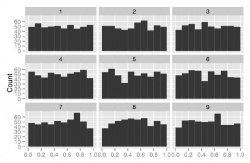
The Rorschach protocol (named after the Rorschach test, in which a subject has to interpret abstract ink blots) is used to calibrate the analysts intuition by showing only null plots.
An example of such a Rorschach is given in Figure 1: Nine histograms summarizing the accuracy at which 500 participants perform nine tasks. What do you see?
The goal of this operation is to train the senses to random deviations, and therefore reduce the effect of apophenia for the given type of visualisation. Although, in order to keep the analysts alert, plots of the real data may be interspersed.
Line-Up

The idea behind line-up (named after the police lineup) is showing the real data plot camouflaged by decoys. In case the observer is able to identify the real data, we can assume that it differs from the null plots. The line-up procedure consists of the following steps:
- generate n - 1 decoys (null datasets)
- make a plot of the decoys and the real data (positioning the real data plot ranomly)
- let an observer assess which plot shows the real data.
The probability (p-value) of such a line-up is easily calculated. A practicable n of 19 leads to a probability of 1/20 = 0.05 (classical p-value) to pick the right plot by chance. To generate even more precise p-values the judge (single observer) can be replaced by a jury.
It is desireable to perform the test in a double-blind environment with neither the observer(s) nor the administrator knowing the true plots. If one has not seen the data yet a self-administered test is possible. Following software was implemented to assist such a procedure.
Software
The above mentioned protocols have been implemented by the authors as an R-package called Nullabor. This package is available for download (as of 16 November 2010).
External Links
Statistics
- General overview of statistics (en.Wikipedia.org)
- Statistical hypothesis testing (en.Wikipedia.org)
- The null hypothesis (en.Wikipedia.org)
- Normal distribution (en.Wikipedia.org)
- Binomial distribution (en.Wikipedia.org)
- Official R-homepage
- Download-site for R-package Nullabor, last accessed November 16, 2010.
Other
- A Sesame Street interpretation of the line-up
- Interactive presentation of [Wickham et al., 2010]
References
- [Wickham et al., 2010] Hadley Wickham, Dianne Cook, Heike Hofmann, and Adreas Buja. Graphical Inference for Infovis. IEEE Transaction on Visualization and Computer Graphics, 16(6):973-979, November/December 2010
- [Scheidegger, 2010] Carlos Eduardo Scheidegger. visualization, etc. - scivis, data vis, infovis and other. Posted on October 24, 2010. Last access on November 17, 2010. URL: http://carlosscheidegger.wordpress.com/2010/10/24/visweek-papers-2-graphical-inference-for-infovis/