Teaching:TUW - UE InfoVis WS 2007/08 - Gruppe 03 - Aufgabe 1 - Volume Visualization

Definitions

• "A Survey of Algorithms for Volume Visualization", [T. Todd Elvins, 1992]

Different slices from a CT scan

Direct Volume Rendering

Introduction

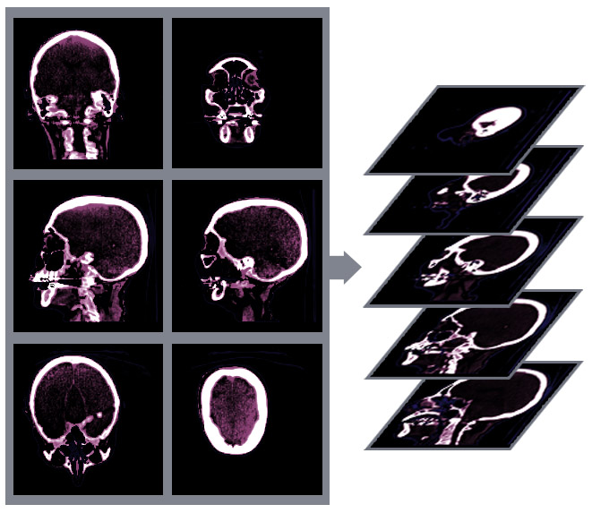
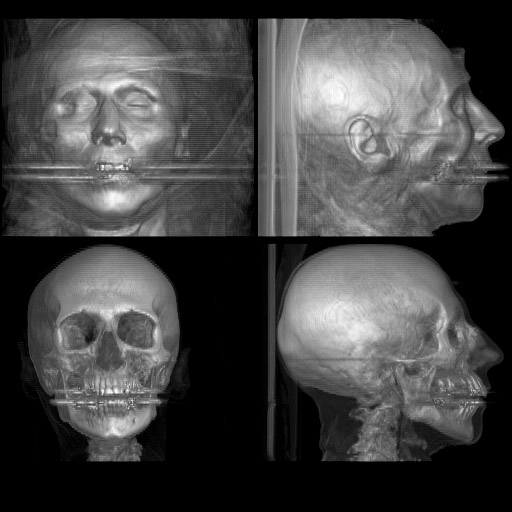
Volume Visualization is the process of understanding multidimensional dataset by projecting it onto 2D images. Generally, the different techniques of Volume Visualization consist of projecting 3D dataset onto 2D images. Those techniques are used in many domains such as medicine, geoscience, astrophysics, chemistry, microscopy and mechanical engineering. "Computed tomography (CT) and magnetic resonance (MR) scanners can be used to create a volume by imaging a series of cross sections."[Drebin et al., 1988]. For example, with a CT scan, we obtain a lot of images which are layers of the head. After a projection, we can obtain different kinds of images, depending on what we want to see.

There are different algorithms for Volume Visualization, the basic steps for all of those algorithms are:

1. Data acquisition either via empirical measurement or computer simulation.
2. Put the data into a format that can be easily manipulated.
3. The data is mapped onto geometric or display primitives.
4. The primitives are stored, manipulated, and displayed.

The different methods for Volume Visualization

There are two fundamental algorithms for Volume Visualization:

1. Direct volume rendering (DVR) algorithms.
2. Surface-fitting (SF) algorithms.

Direct Volume Rendering

DVR methods map elements directly into screen space without using geometric primitives as an intermediate representation. These methods are effective with amorphous features such as clouds, fluids, and gases.These methods have one disadvantage, they need to traverse all the dataset for each rendered image, and each recalculation can be time-consuming. There is a solution to avoid this problem : the "progressive refinement". It consists of creating a low resolution image and then refining it by increasing the resolution and the quality.

Surface-Fitting

SF methods are also called feature-extraction or iso-surfacing and fit planar polygons or surface patches to constant-value contour surfaces. SF methods are usually faster than DVR methods since they traverse the dataset once, for a given threshold value, to obtain the surface and then conventional rendering methods (which may be in hardware) are used to produce the images. New views of the surface can be quickly generated. Using a new threshold is time-consuming since the original dataset must be traversed again.

References

• [Elvins, 1992] T. Todd Elvins. A survey of algorithms for volume visualization. Computer Graphics 26:3, pp. 194-201, August 1992, http://portal.acm.org/citation.cfm?id=142427
• [Drebin et al., 1988] Robert A.Drebin, Loren Carpenter, Pat Hanrahan. Volume Rendering. Computer Graphics 22:4, pp. 65-74, August 1988, http://portal.acm.org/citation.cfm?id=378484.