Teaching:TUW - UE InfoVis WS 2007/08 - Gruppe 01 - Aufgabe 1 - View Relationships

View Relationships

[Drakos and Moore] Nikos Drakos and Ross Moore 1993-1999, translated by Niki Sahling 2002.12.03, Interactive 3D Scatterplots - From High-Dimensional Data to Insight, http://www.vrvis.at/via/resources/DA-NSahling/node2.html

Up to three relationships are shown in the 3D scatterplot per se, this is extended across multiple views by visual cues, i.e. color and motion, and linking and brushing. Relations in the data space can be characterized by their dimensionality. A two-dimensional constraint means that an attribute a_2 is dependent of one other attribute a_1: f{(a_1,a_2)}=0. This is a simple constraint which can be shown in every 2D diagram. A 1D constraint in 3D space f{(a_1,a_2,a_3)}=0 forms a surface in 3D space. The mapping to a 2D visualization may result in a view where the characteristics of the higher-dimensional relation are not visible anymore - the viewer may not find them. Obviously nD relations can be directly shown in nD space, and only with strong limitation in (n-1)-dimensional visualization.

With common 2D techniques, the ability to show relations is restricted to 2D, but multiple views and linking can provide a substitution. With 2D scatterplot-matrices linking supports exploration of nD relations, but it can not establish a 3D impression of relations. With 3D scatterplots relations up to the third dimension can be shown, and with linking, the possibilities are even extended. Of course, the extension from 2D to 3D looks small under the circumstances of nD data and n grows up to 20 or 25. But the higher the dimensionality of the relation is, the less is its commonness and the benefit from its interpretation. It is harder to interpret such relations and does not support insight as high-dimensional objects are hard to grasp.

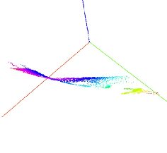
An attribute which shows dependencies to a combination of two others (a 3D surface or similar structure) will appear as a 3D structure in the 3D scatterplot. Figure 1 shows an example of such a structure, the relation is shown from different viewpoints of a three-dimensional representation. The interpretation is also rather straightforward as the user can see the 3D structure and analyze it. This is an obvious advantage to a 2D visualization, because a 3D surface is difficult to find in 2D space.

Figure 1 pressure (green), absolute-pressure (red), and velocity (blue) result in a surface in 3D (shown from different viewpoints). Obviously the relation between pressure and absolute-pressure is not linear (shown in the right plot).

Figure 1: pressure (green), absolute-pressure (red), and velocity (blue) result in a surface in 3D (shown from different viewpoints). Obviously the relation between pressure and absolute-pressure is not linear (shown in the right plot).

This can be further extended, if the 3D structure is not clear and outliers are more common, brushing and linking can show that there is another parameter that influences the relation. Brushing the outliers and isolating them from the assumed relation can show another dependency in a linked view. This can be continued, but the relation is getting harder to understand with every additional dimension which is not shown in the same view.

Linking and brushing in multiple views is a useful tool to analyze relations, because the human perception system recognizes color highlighting very efficiently. Color can be used as a visual cue, not only with highlighting, if the same attribute is mapped to the color value in different views, the affiliations can be perceived across multiple views. Another visual cue which works in the described environment is motion. The 3D rotation of the scatterplot moves the data point with different speed according to the position (front or rear), so neighbors are moving with similar speed which can be easily detected. This cue also works beyond different views, if the rotation is coupled, and the movements are smooth.