Social Network Generation: Difference between revisions
m Reverted edit of WjcNqk, changed back to last version by Markus |
added to coffee room |
||
| Line 579: | Line 579: | ||
</blockquote> | </blockquote> | ||
[[Category:Datasets]] | [[Category:Datasets]] | ||
[[Category:Coffee Room]] | |||
Revision as of 03:31, 26 March 2008
This wiki page is under construction...
Research work and images have been realised by Nathalie Henry and Jean-Daniel Fekete, using MatrixExplorer, built with the Infovis Toolkit.
Social Network Characterization
Social networks involve persons or groups called actors and relationship between them, with a lot of variety in the kind of actors and relationships. As described in Wasserman and Faust, actors can be people, subgroups, organizations or collectivities; relations may be friendship (relationships), interactions, communications, transactions, movement or kinship. However, the nature of actors and relations does not really matter: we focus on their structure. We can classify the social networks studied in the literature in three categories:
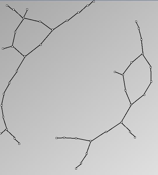
- Tree-like are trees with additional links forming cycles with a specified probability. This category includes genealogy data and very sparse graphs such as Sexually-Transmitted Disease (STD) transmission patterns. We call them “almost trees” because they have are mostly acyclic and nodes have very few parents.
- Almost complete graphs are complete graphs with missing relations. For example, data about trade between countries, cities or companies are almost complete graphs. They are interesting to study as valued graphs; since they usually carry values on their edges.
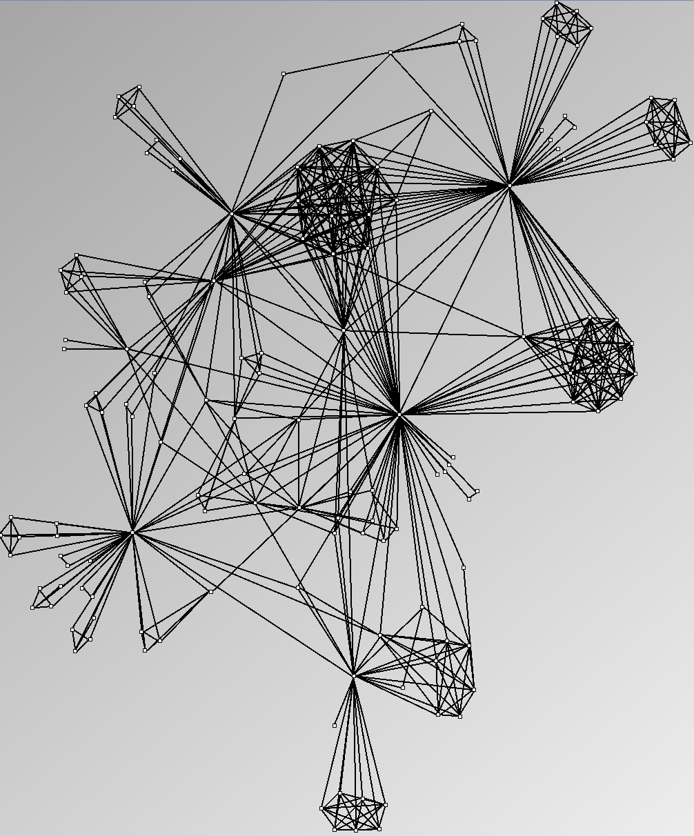
- Small-world networks (also scale-free or power-law degree-distribution networks) have been studied intensely since they were first described in Watts and Strogatz. They defined them as graphs with three properties: power-law degree distribution, high clustering coefficient and small average shortest path. They are locally dense (sparse with dense sub-graphs).
Three methods exist to select datasets for assessing the quality of analysis systems in the context of social networks: selecting one or two real datasets hoping they are representative, selecting several datasets or generating random datasets with well-known characteristics shared by social networks. With this last method, one should generate datasets with a controlled set of properties and evaluate the systems knowing the properties in advance. It should then eliminate biases linked to a particular dataset and eases the replication of experiments. Unfortunately, while generating tree-like and almost-complete graphs is relatively straightforward, generating graphs with a small-world network structure is still a research topic for computer scientists and physicists. This page shows the results of popular and available network generators. In light of the real social networks we present in the #Real Social Networks, we consider them unsuitable for evaluations since users can easily notice their artifical nature.
Issues on Social Network Generation for Evaluating Visualizations
Watts and Strogatz first described in (Watts, D. J. and S. H. Strogatz (1998). "Collective dynamics of 'small-world' networks." Nature 393: 440 - 442) the concept of small-world networks. They formalized these networks as graphs with three properties: power-law degree distribution, high clustering coefficient and small average shortest path. In the same paper they propose a basic model fitting these properties consisting in a grid (fixed local neighborhood) with additional links simulating some unexpected relations support to the six degrees of separation discovered by Milgram (Milgram, S. (1967). "The small world problem." Psychology Today: 60-67). Barabási and Albert proposed an incremental model to improve it (Barabási, A.-L. and R. Albert (1999). "Emergence of Scaling in Random Networks." Science 286(5439): 509 - 512. ). Since Watts and Strogatz’ model, several have been proposed each generating networks with one or two of the described properties (power-law) but none combine the three of them.
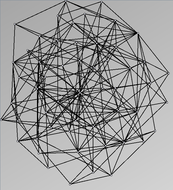
Here are some results of available generators present in the JUNG package. Let's note that for each network generated we only keep the biggest component. Generators present in Pajek[1] and Geomi[2] are incremental scale-free networks generators such as the Barabasi and Albert model.
About datasets and representations
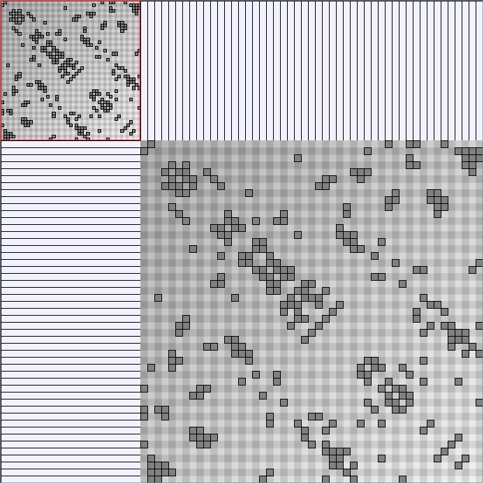
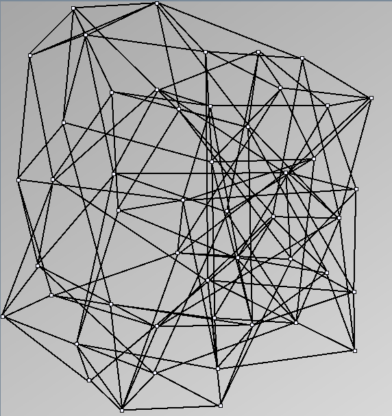
- All datasets are downloadable in GraphMl format.
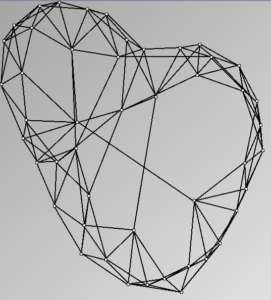
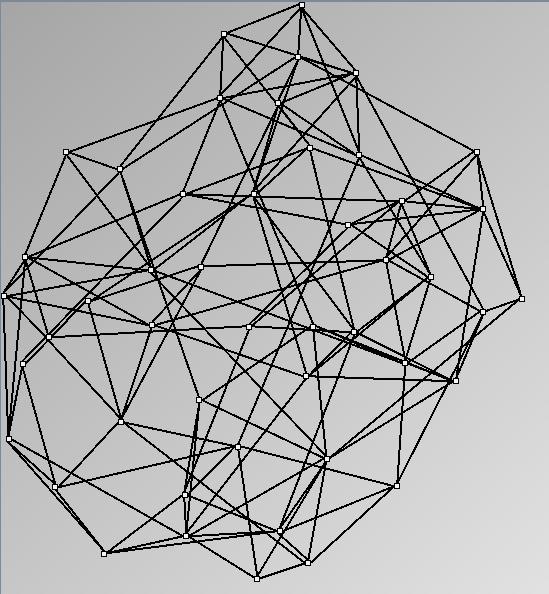
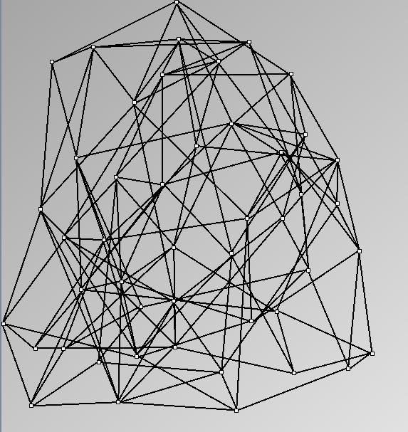
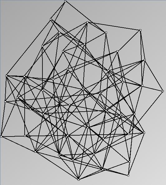
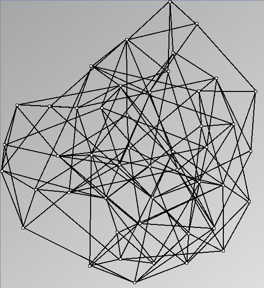
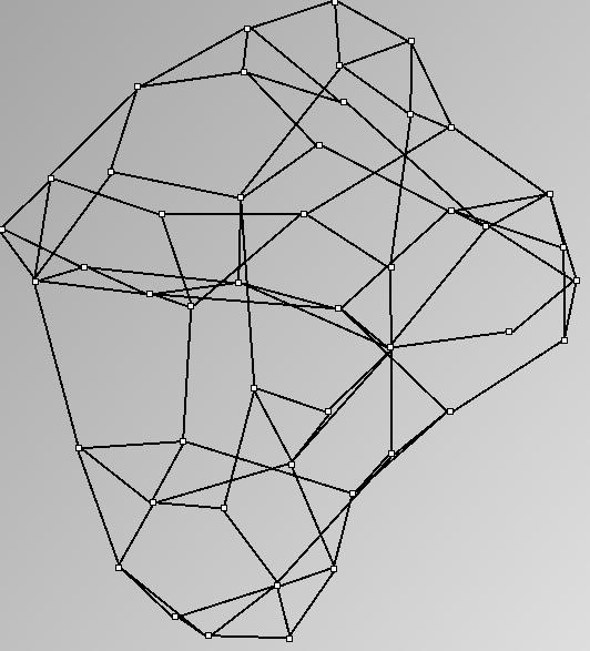
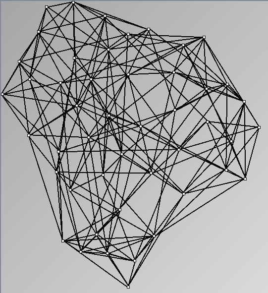
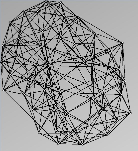
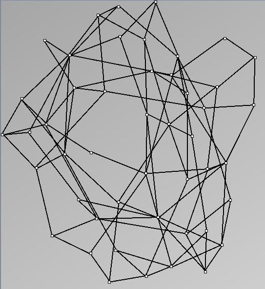
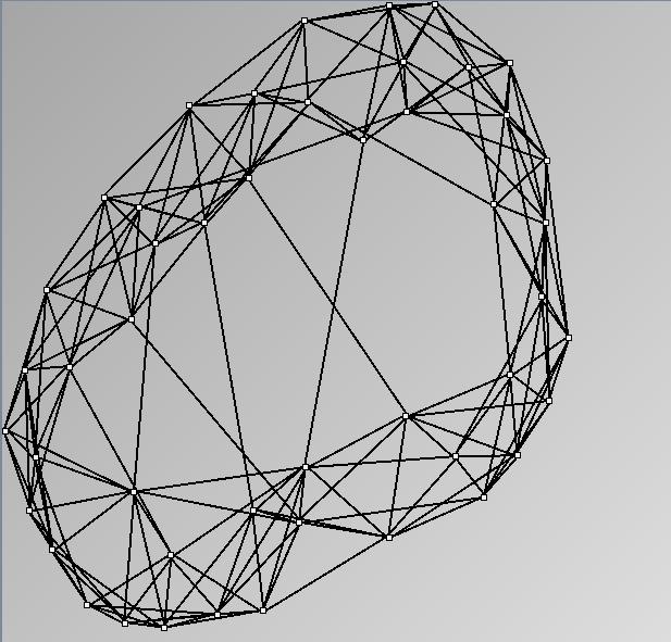
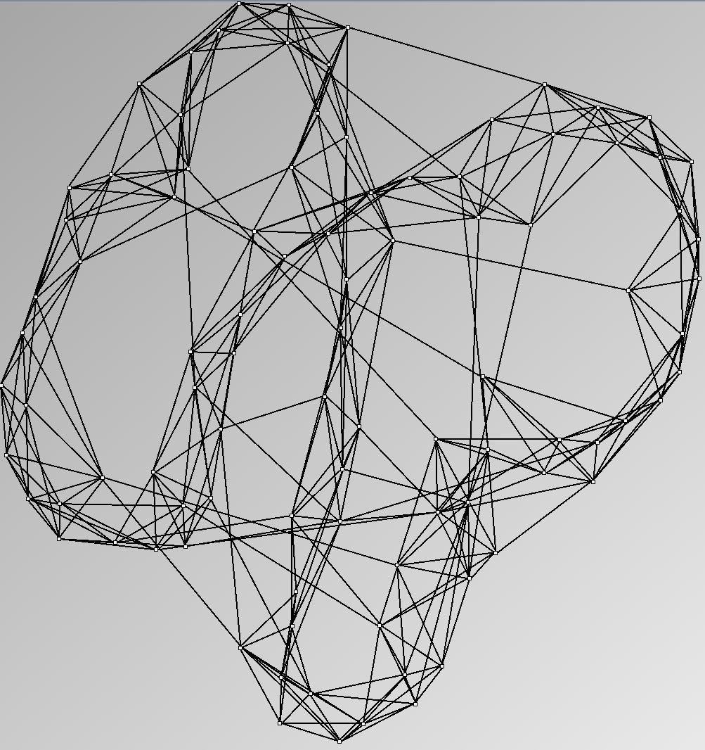
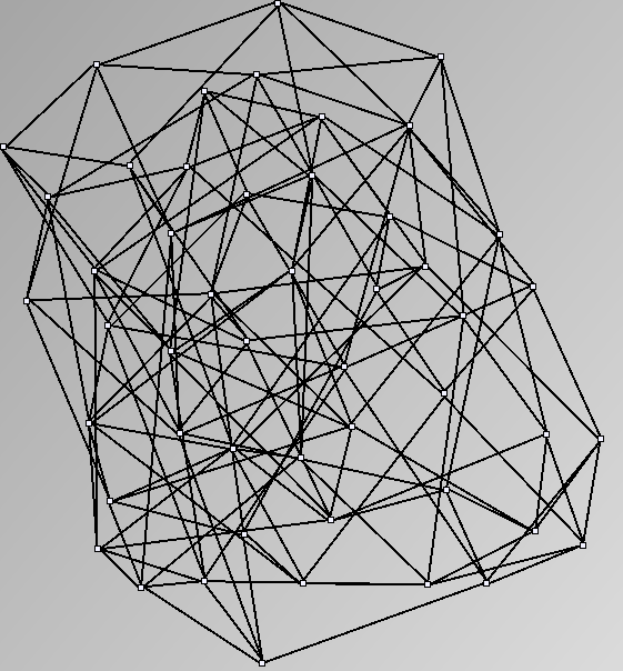
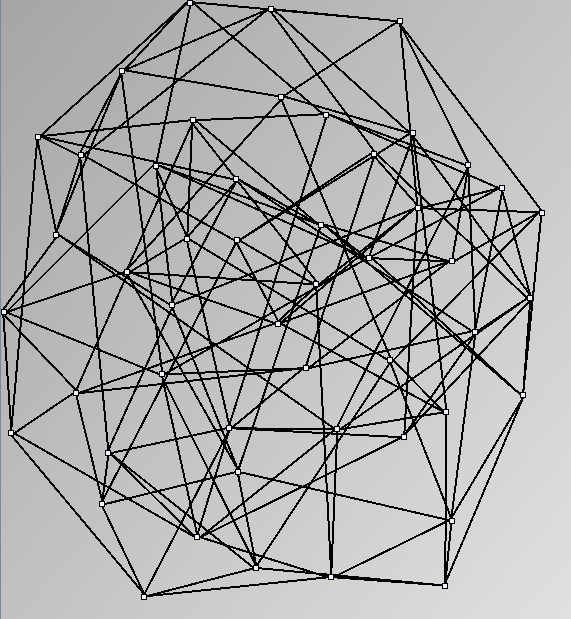
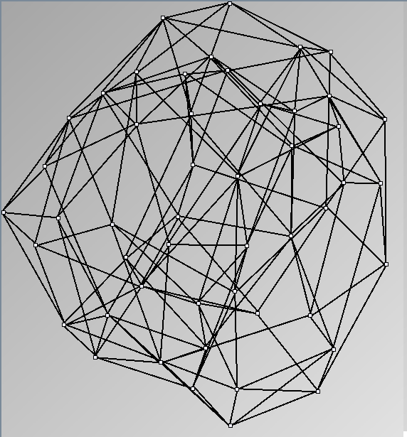
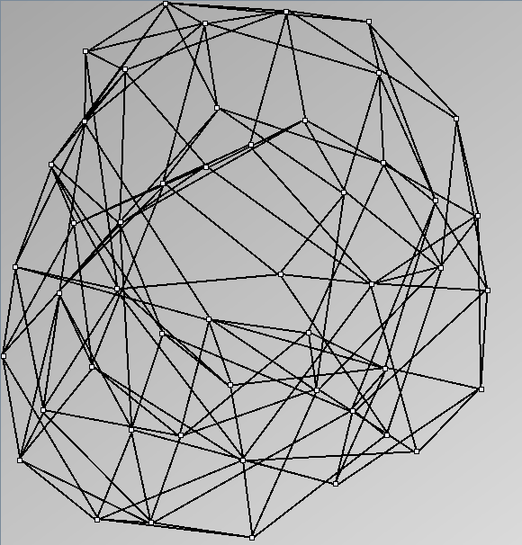
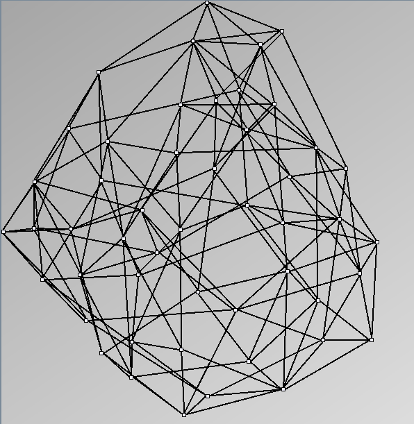
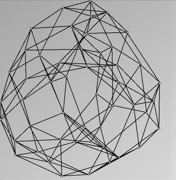
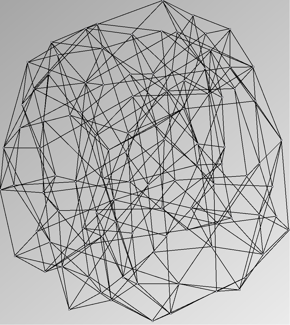
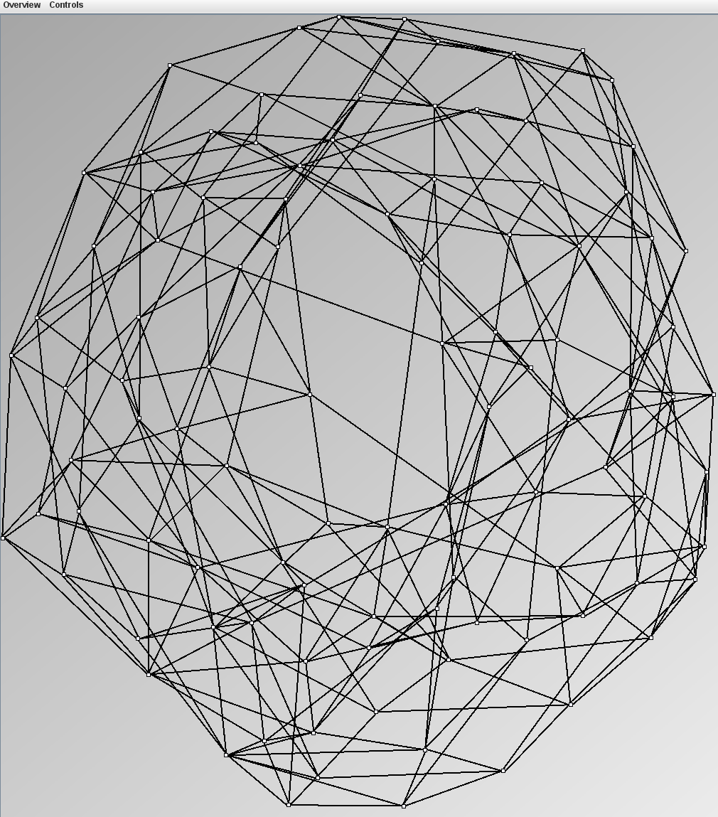
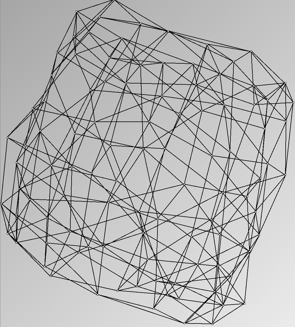
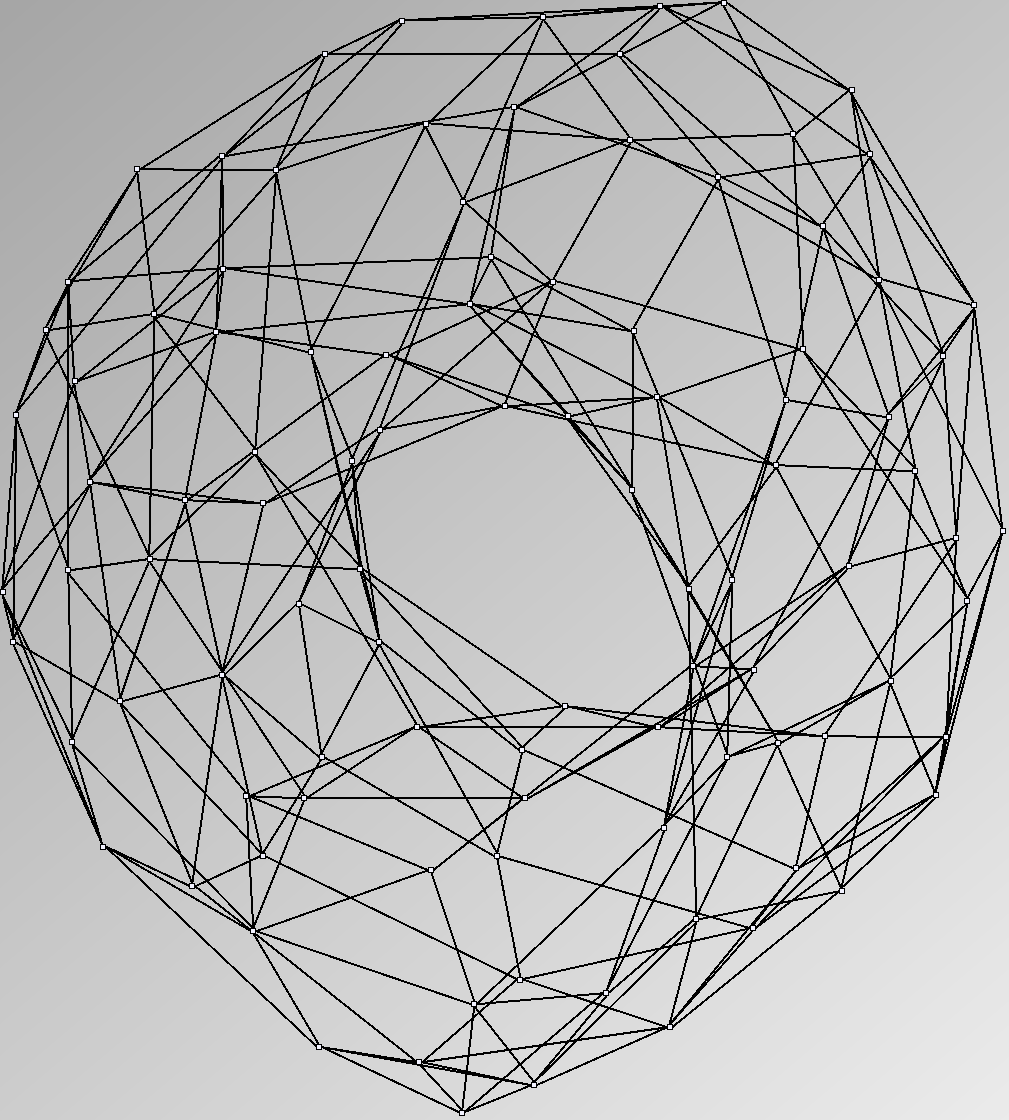
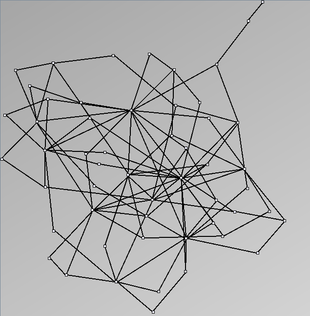
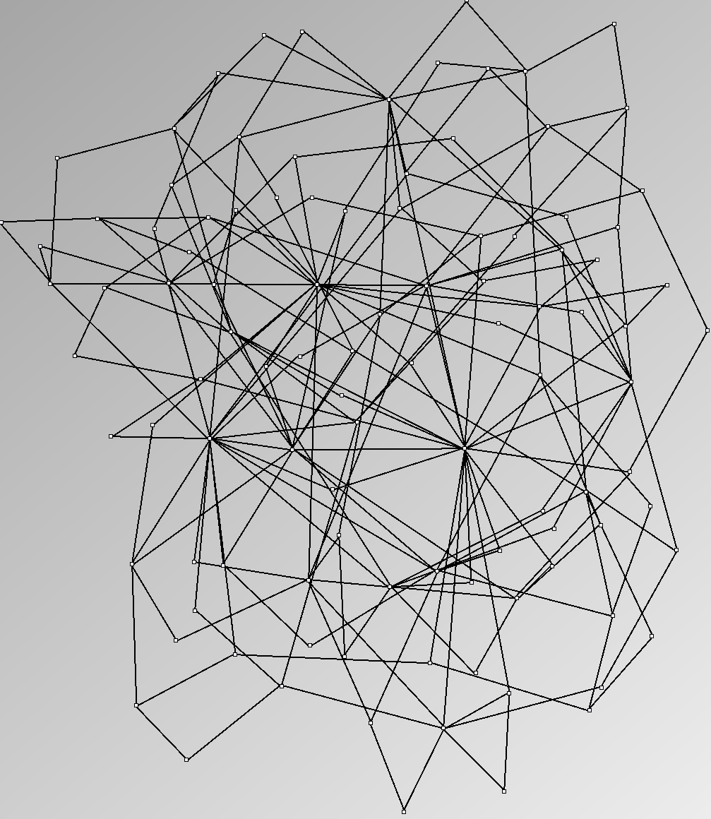
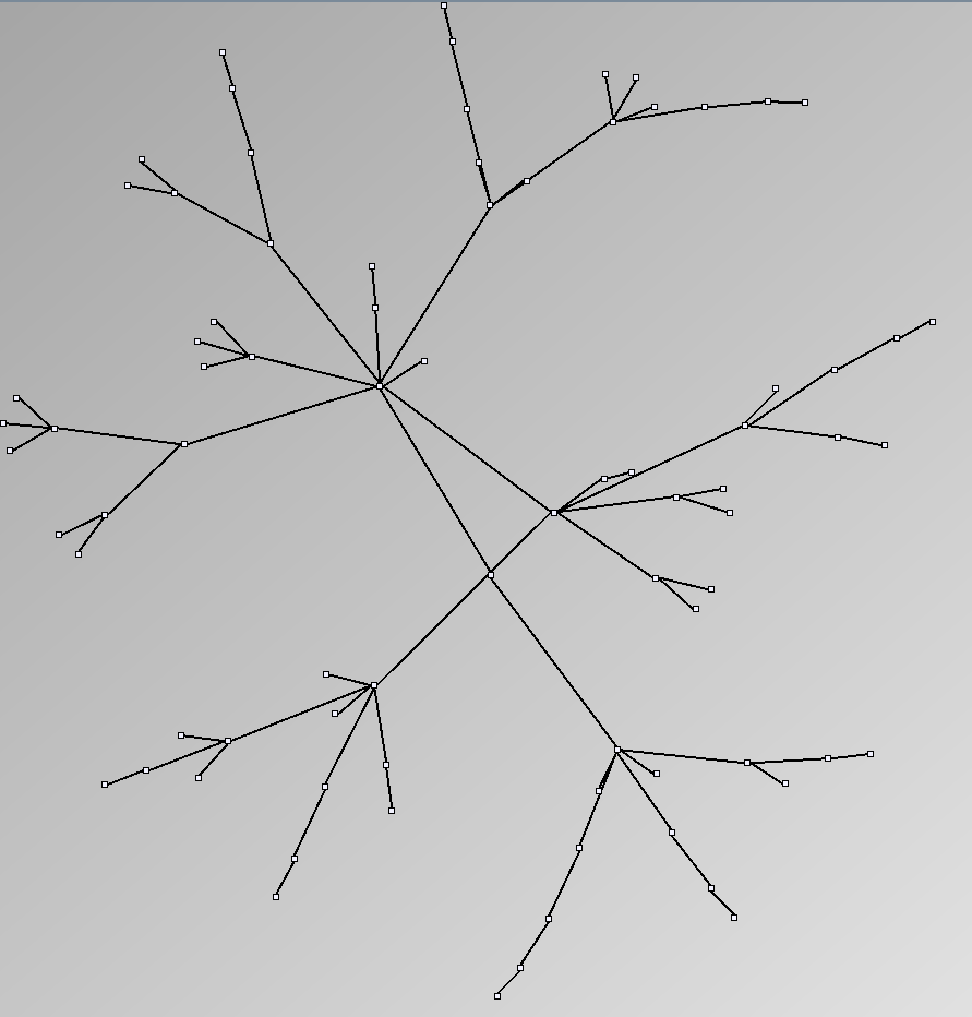
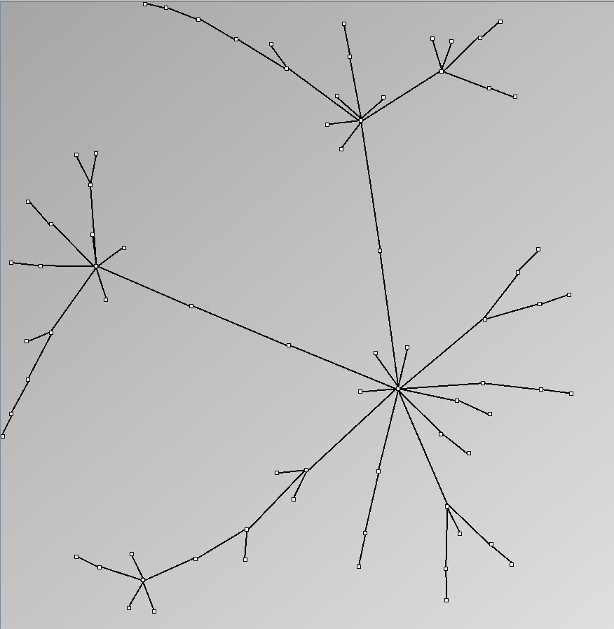
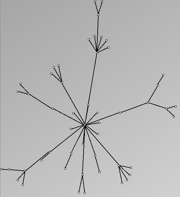
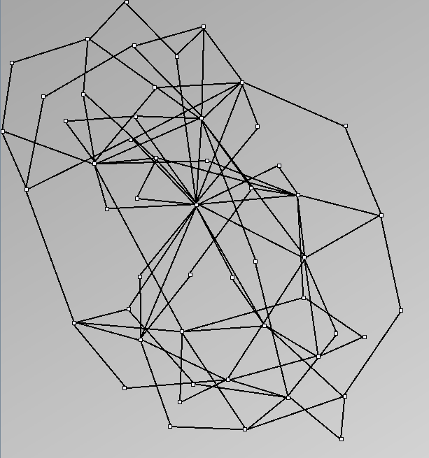
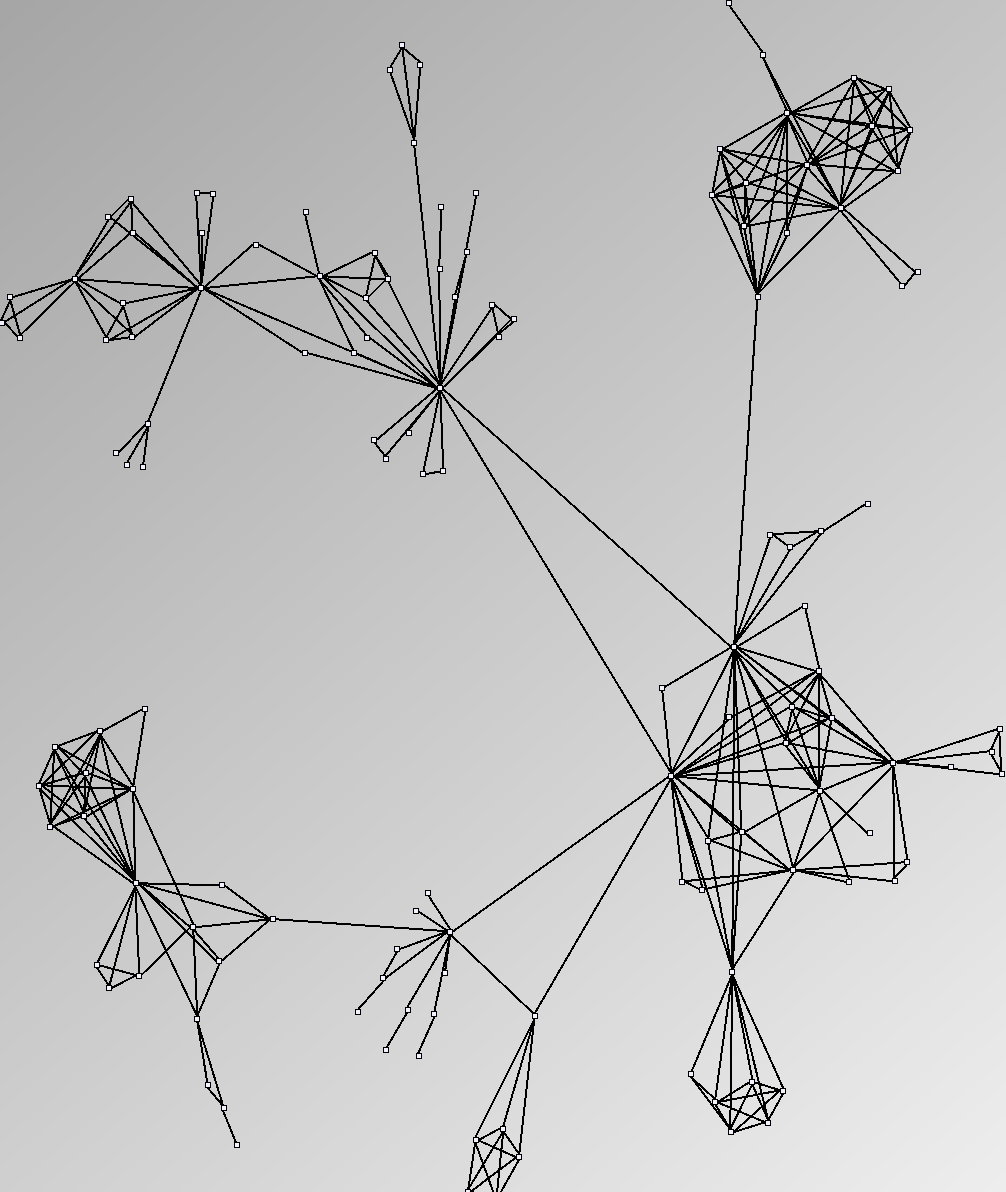
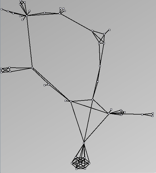
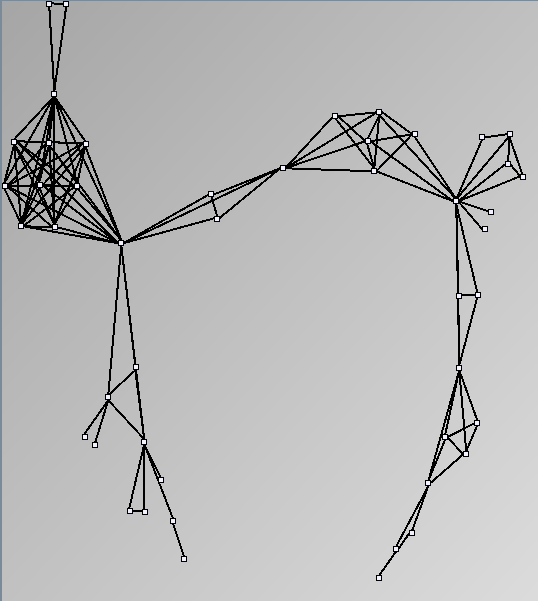
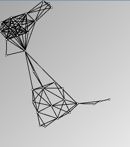
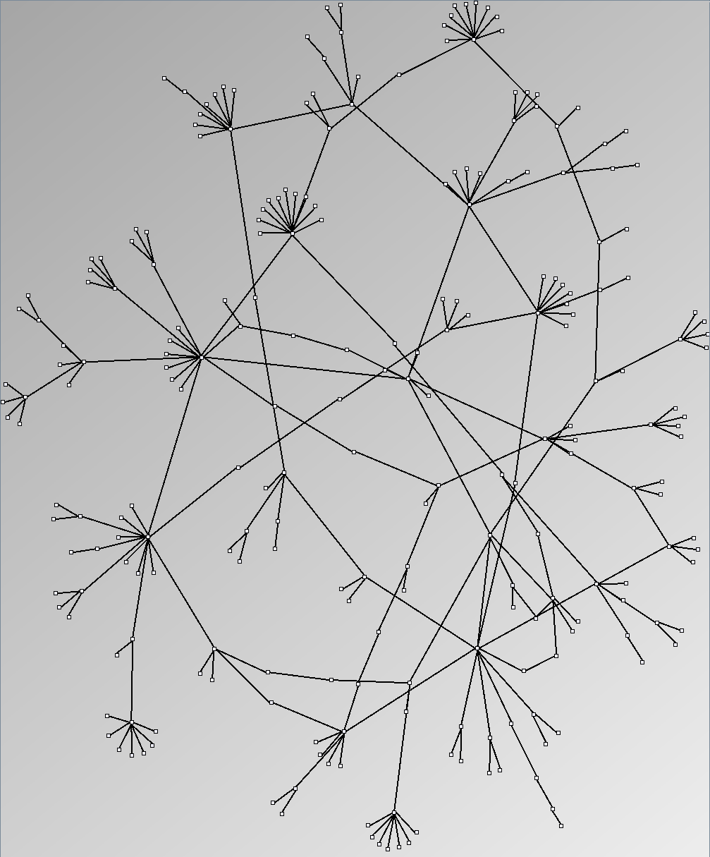
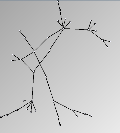
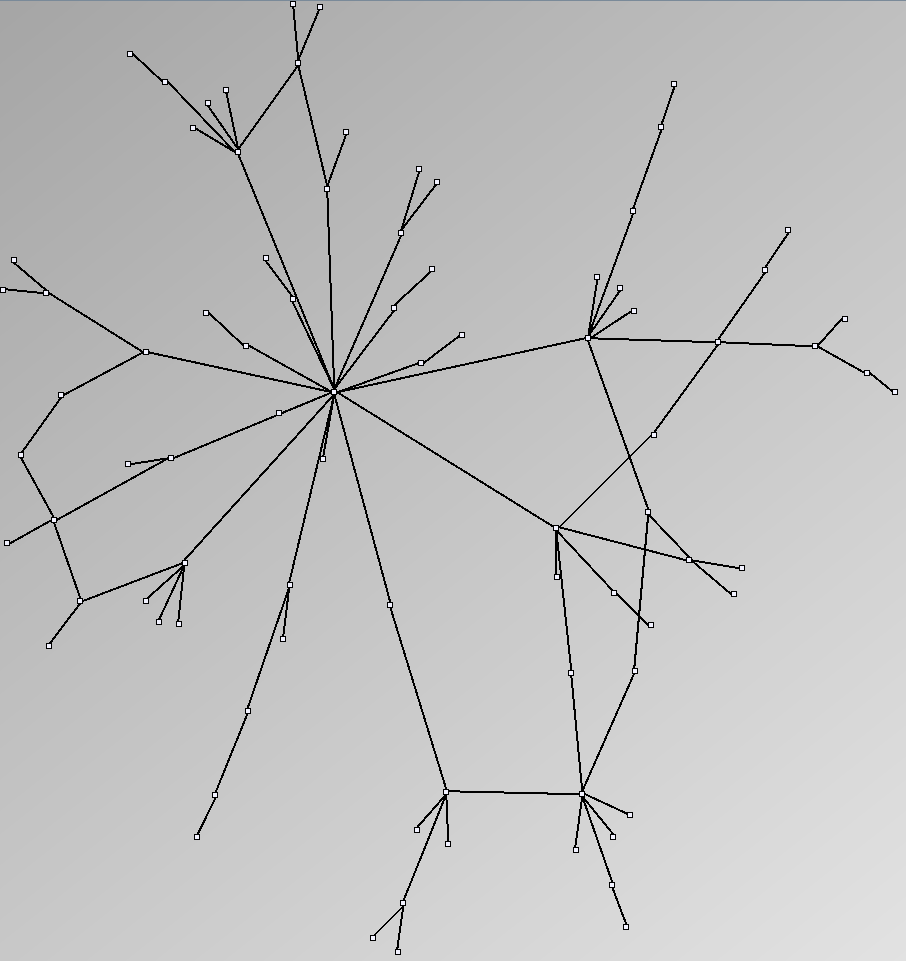
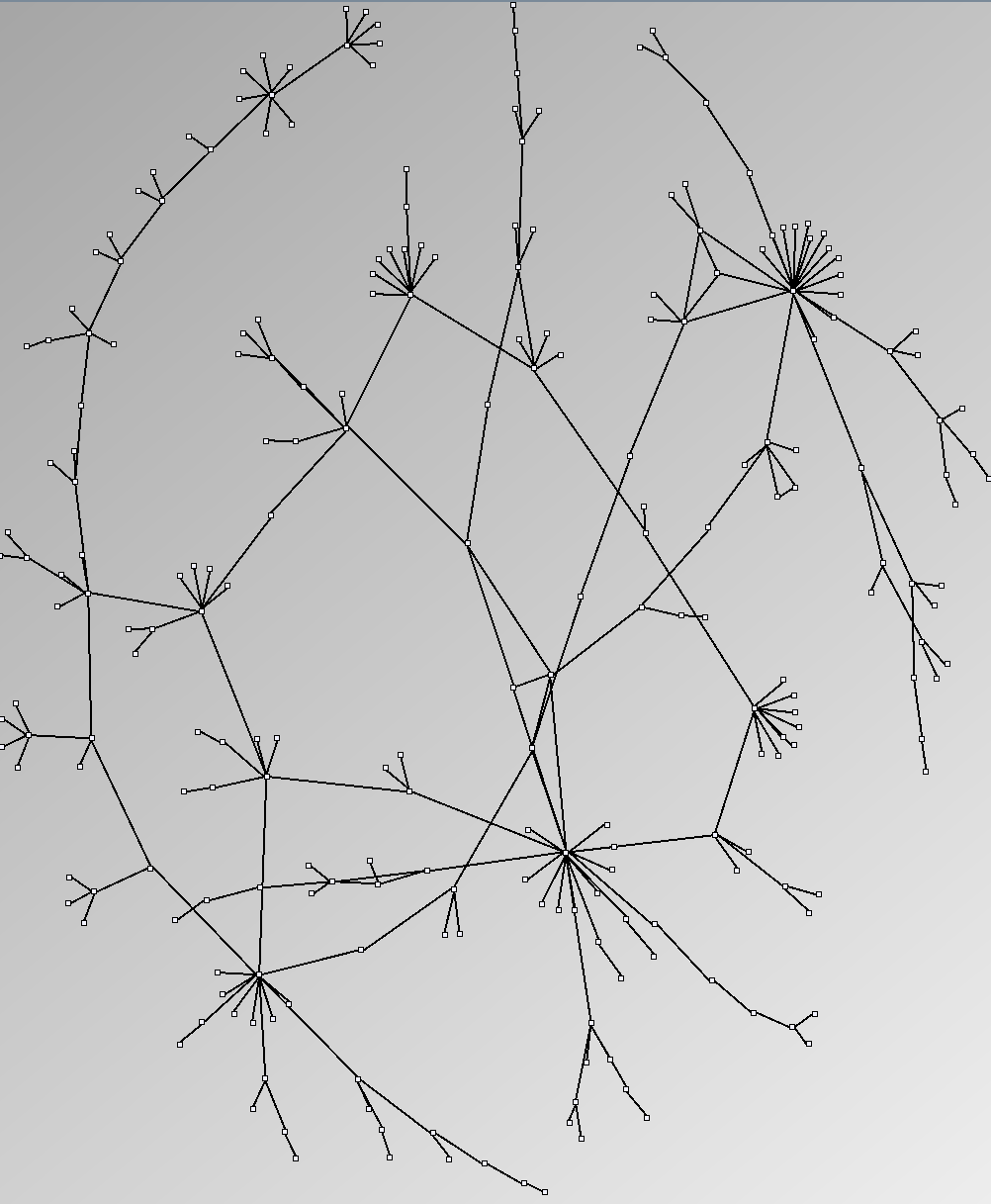
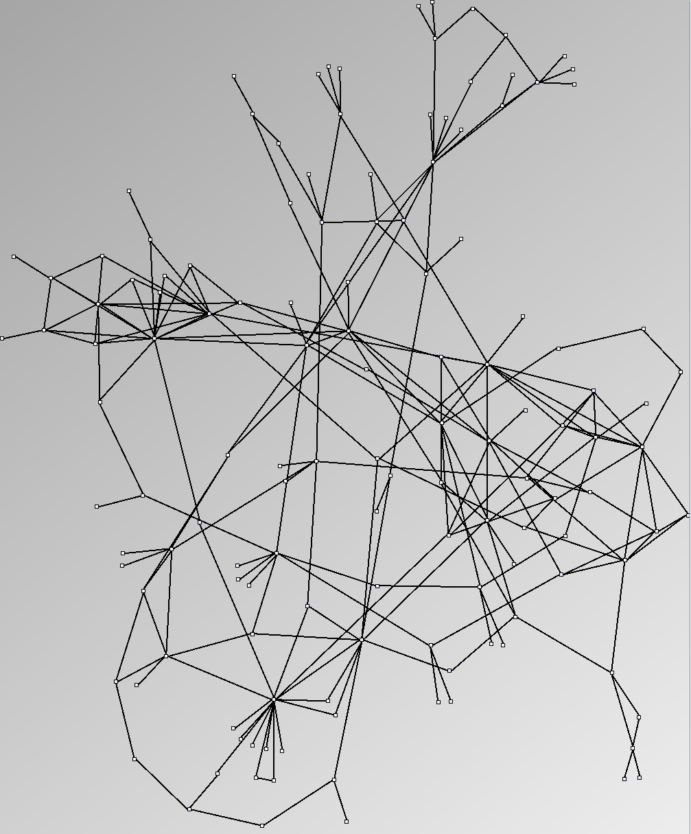
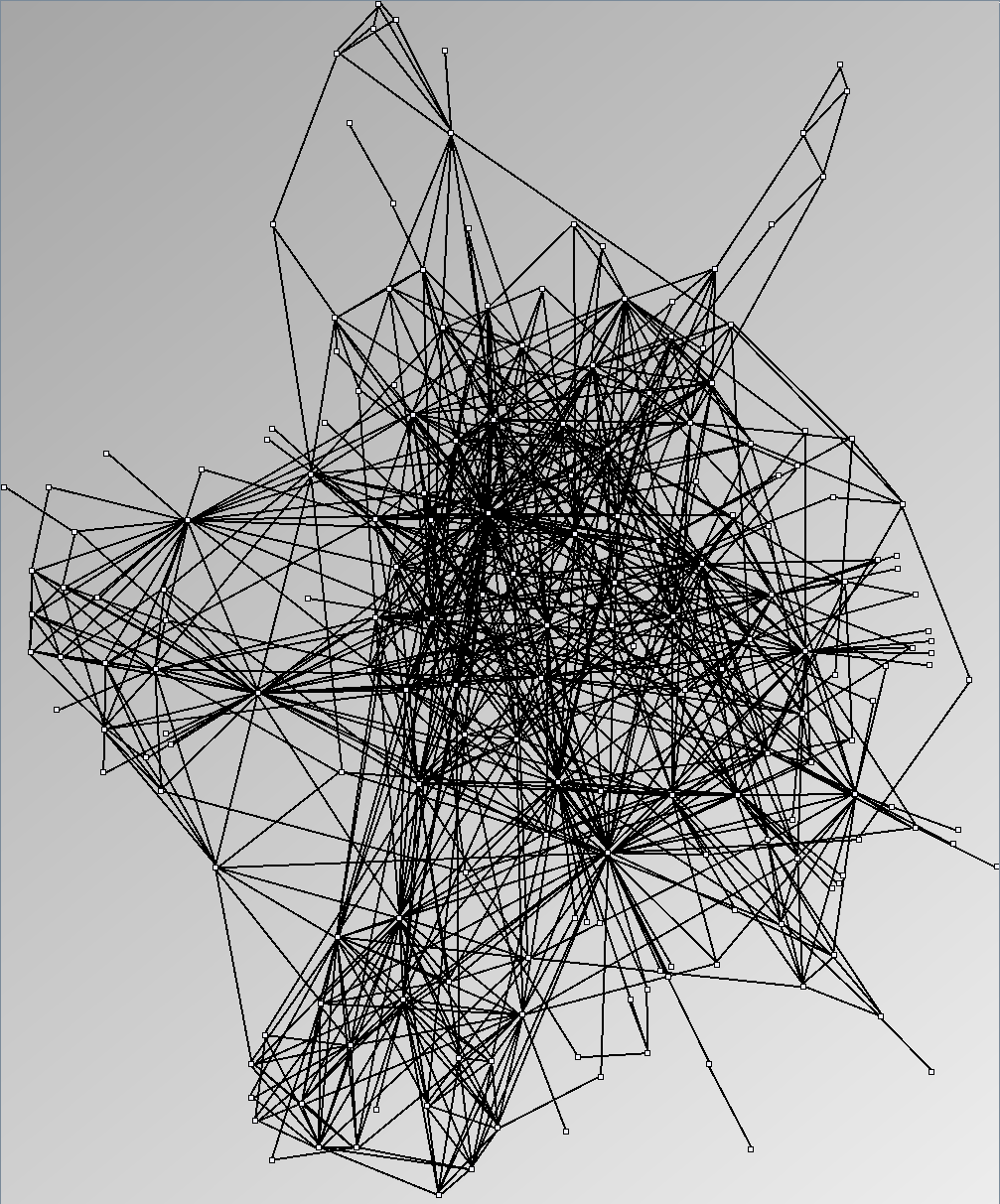
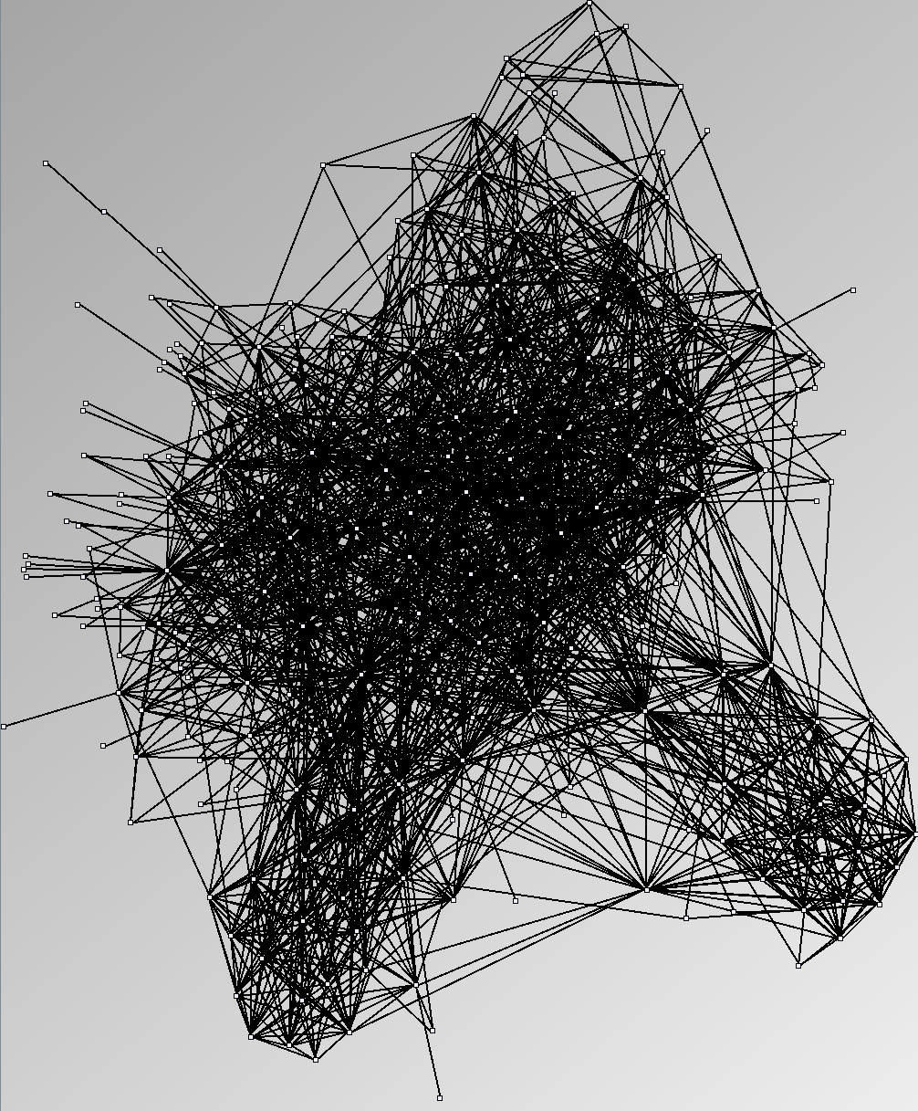
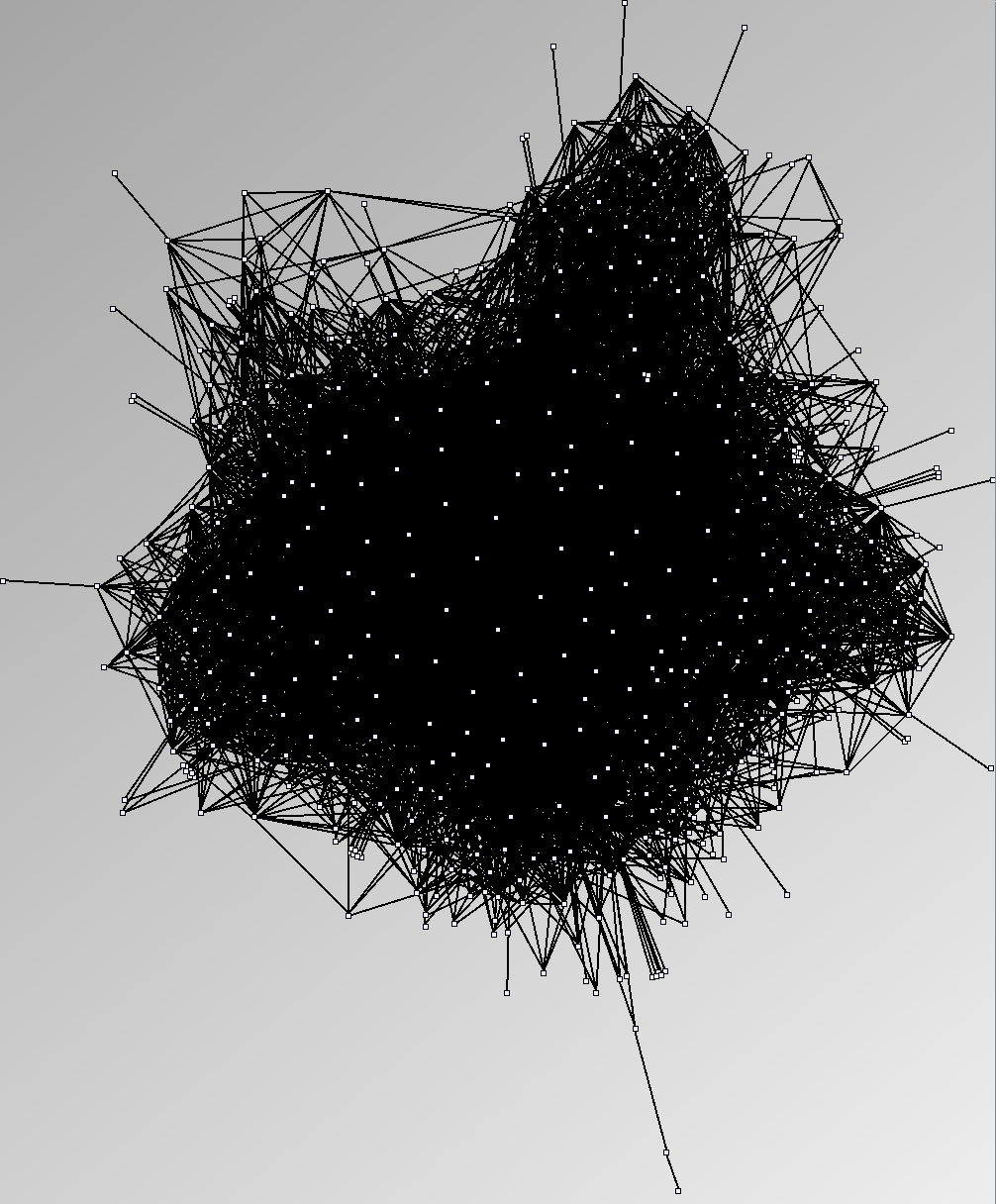
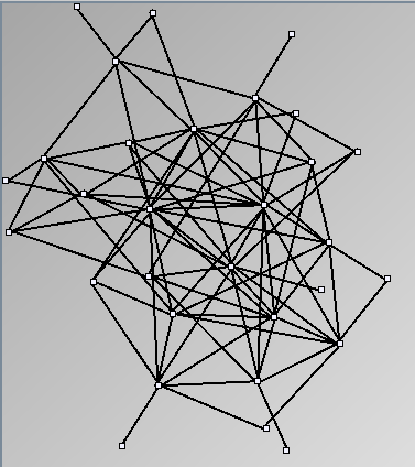
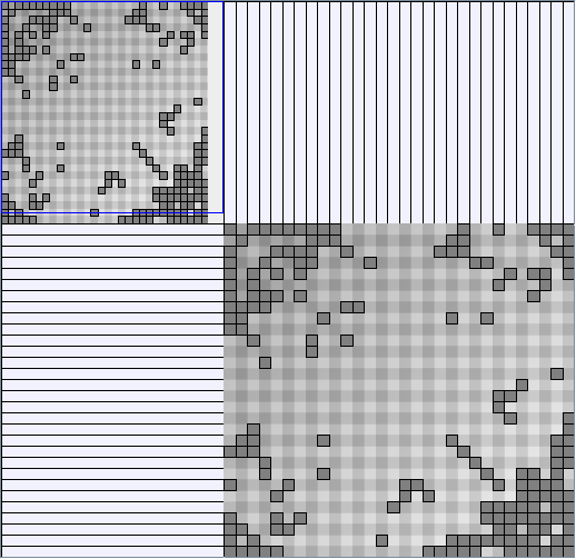
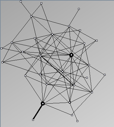
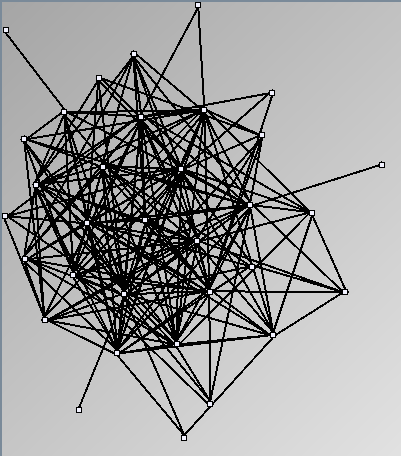
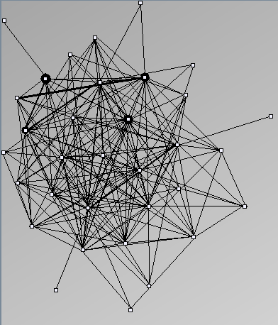
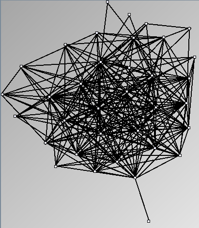
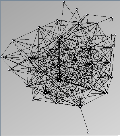
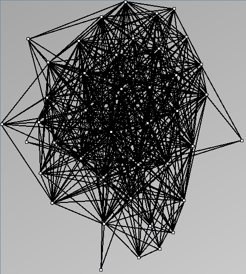
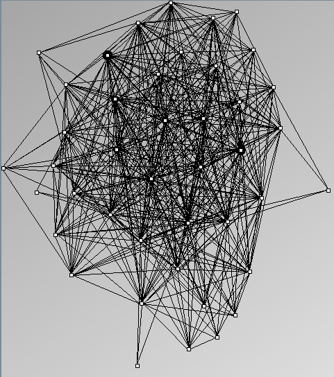
- Node-Link diagrams are ordered with the linLog algorithm of Andreas Noack [Graph Drawing 2005] (with edge-repulsion coefficient of 2.5f).
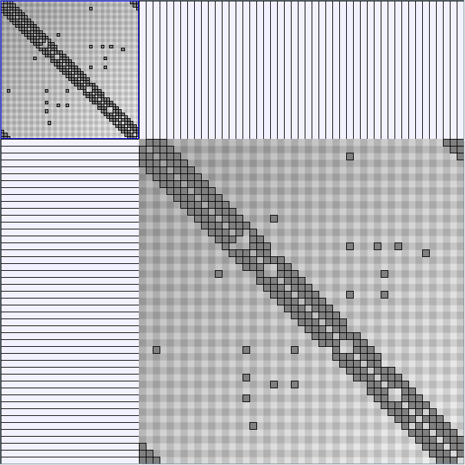
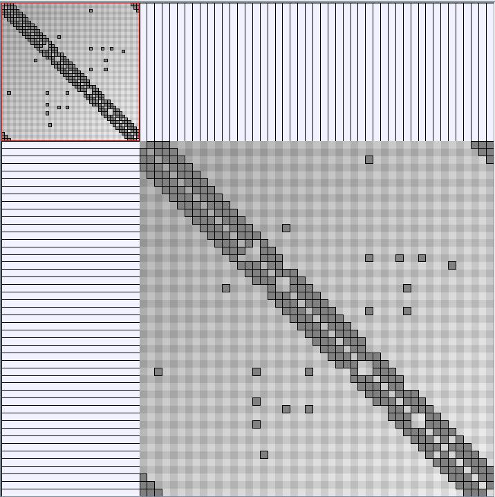
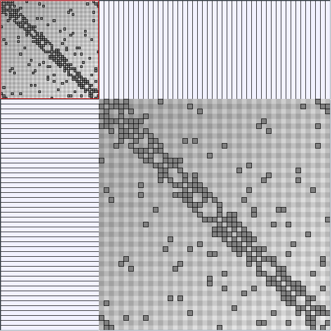
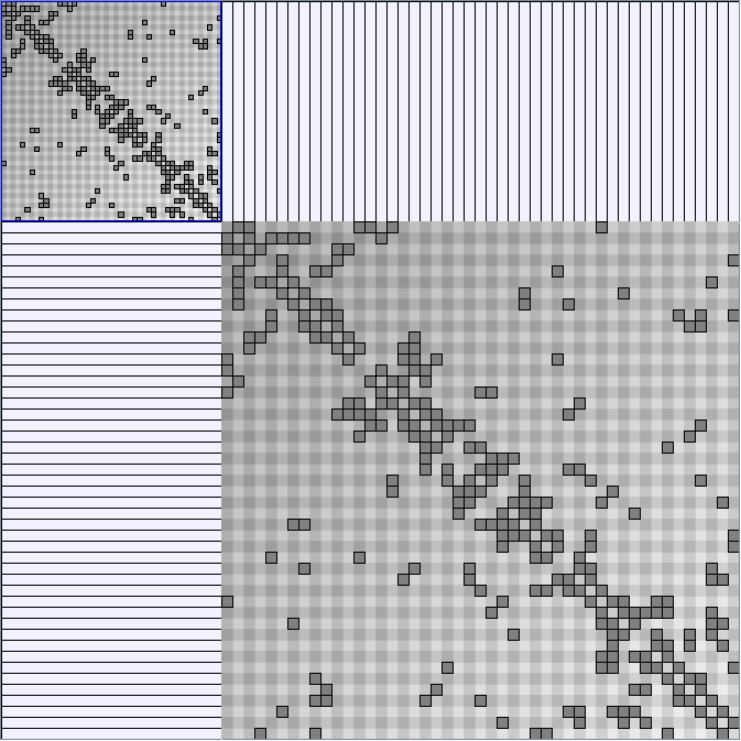
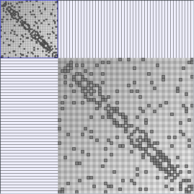
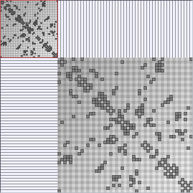
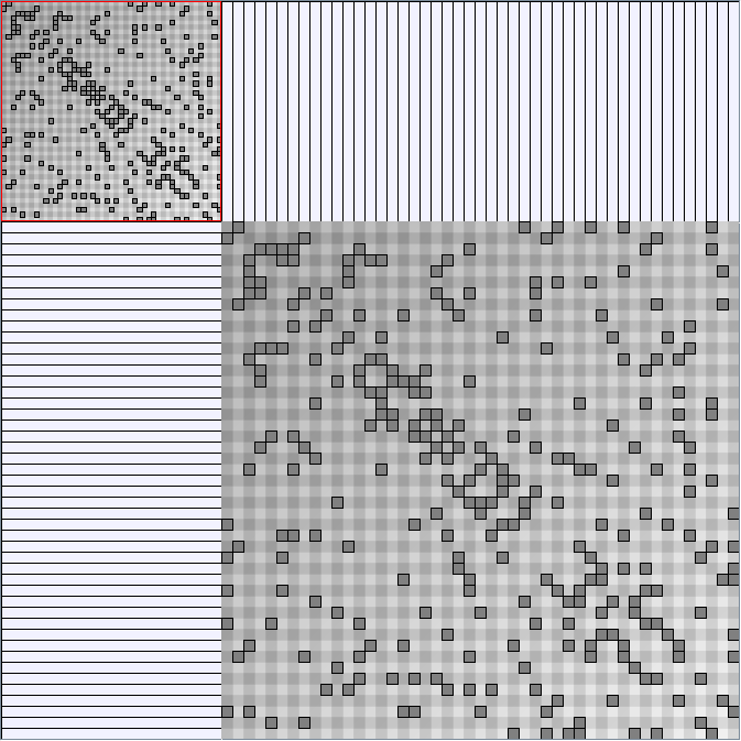
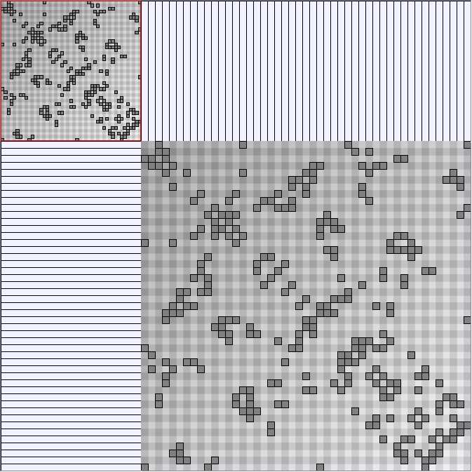
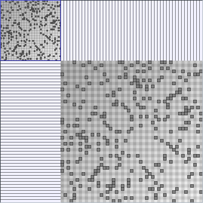
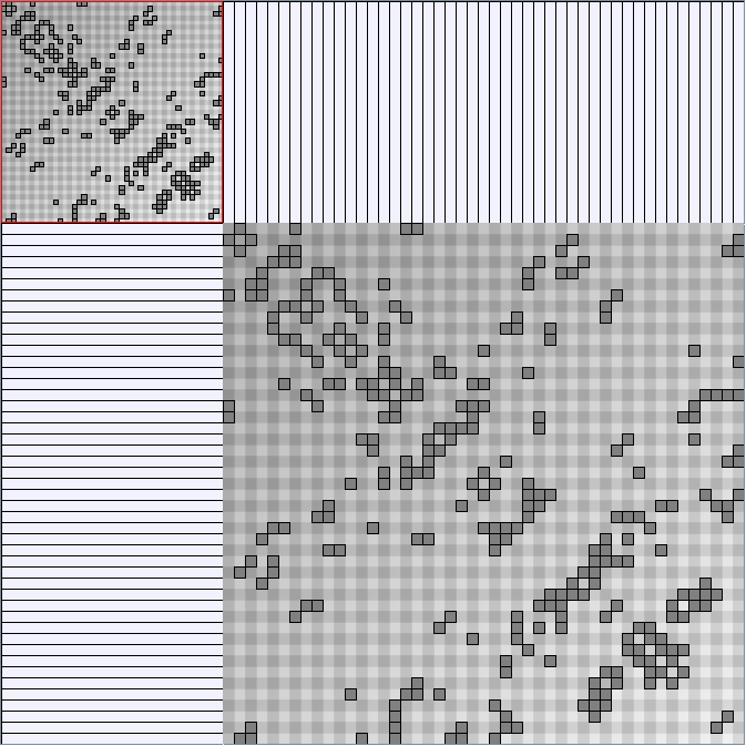
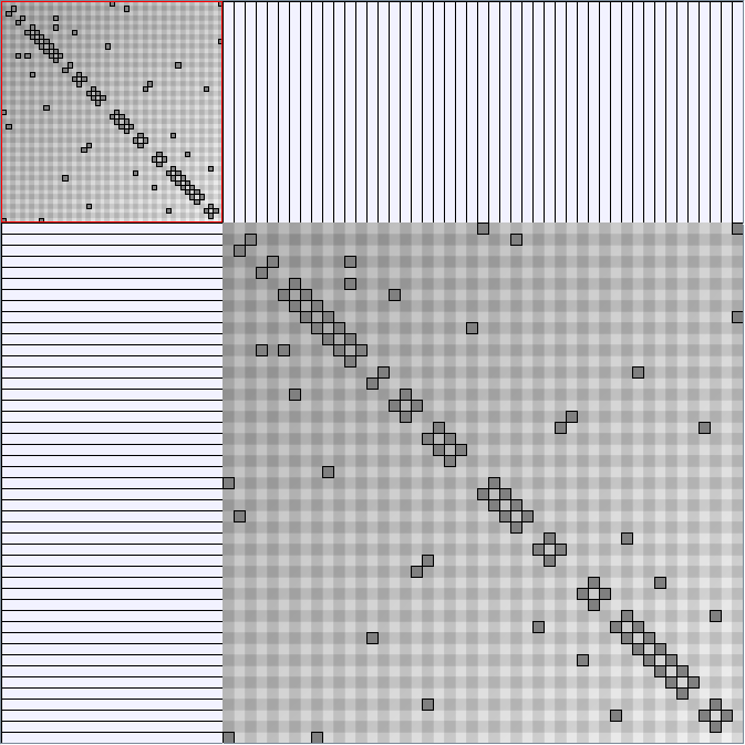
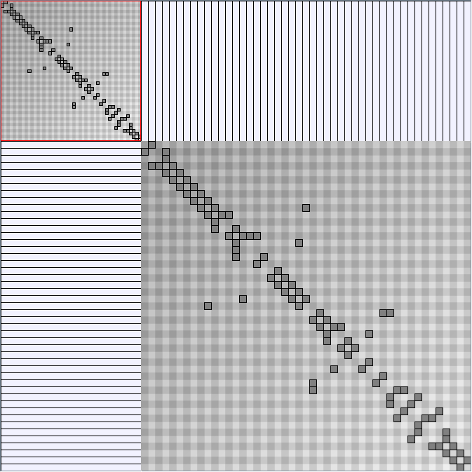
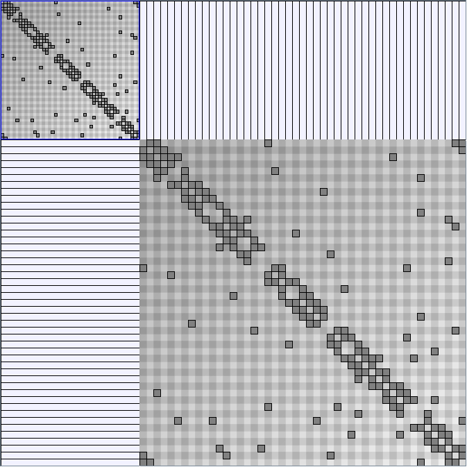
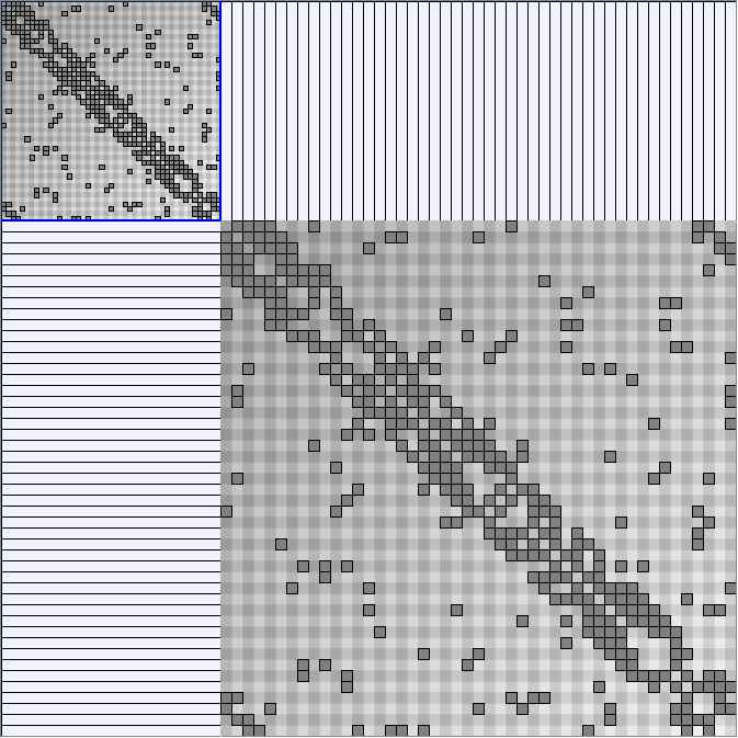
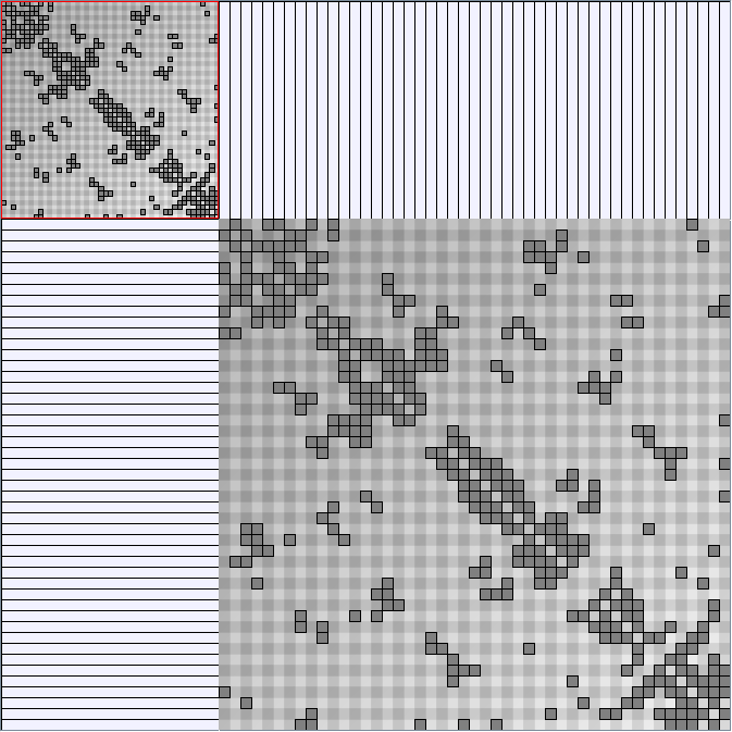
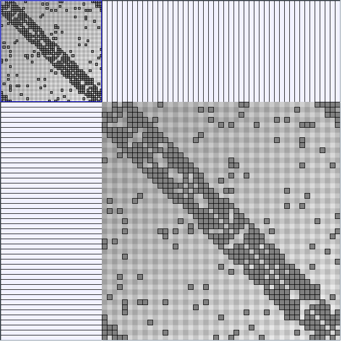
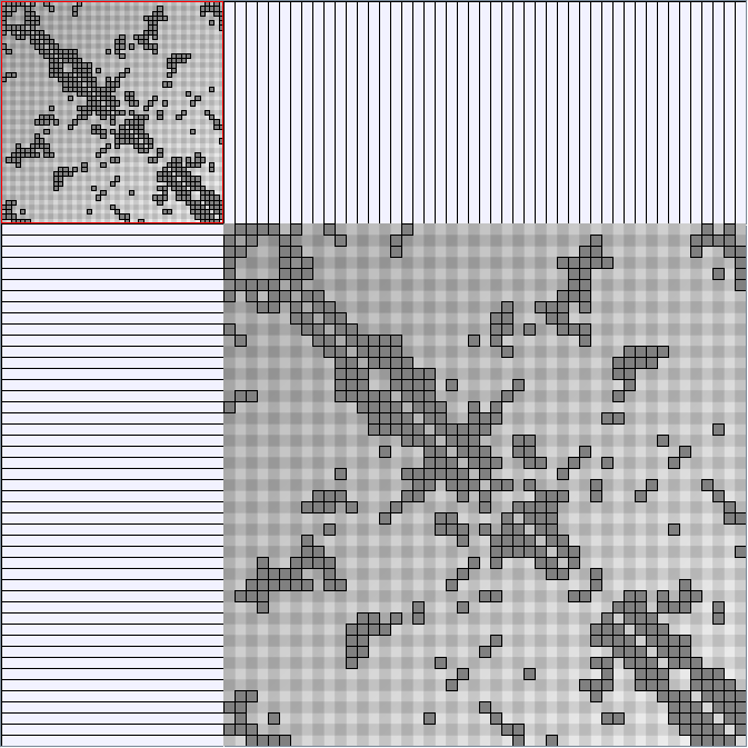
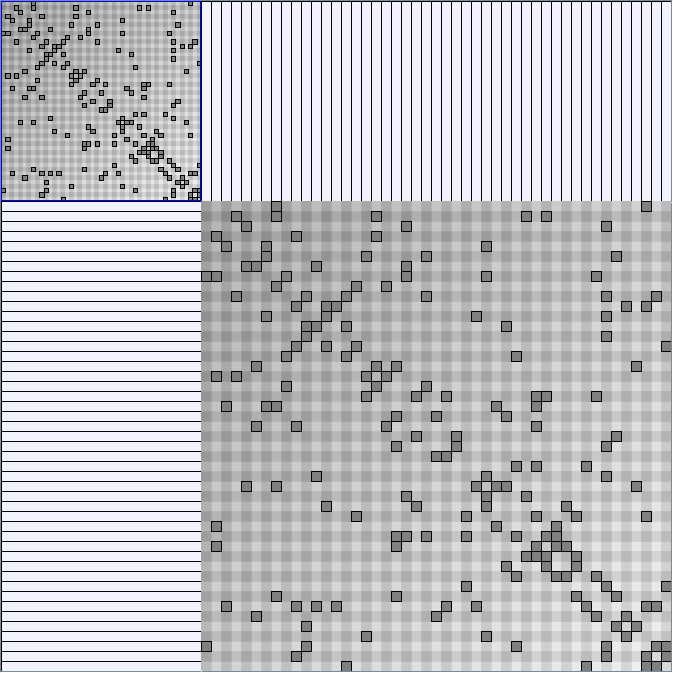
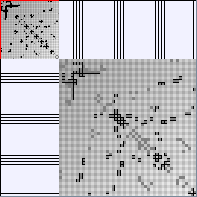
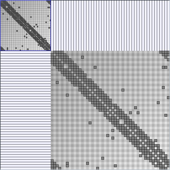
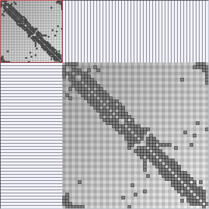
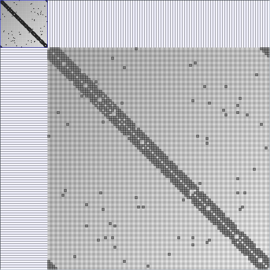
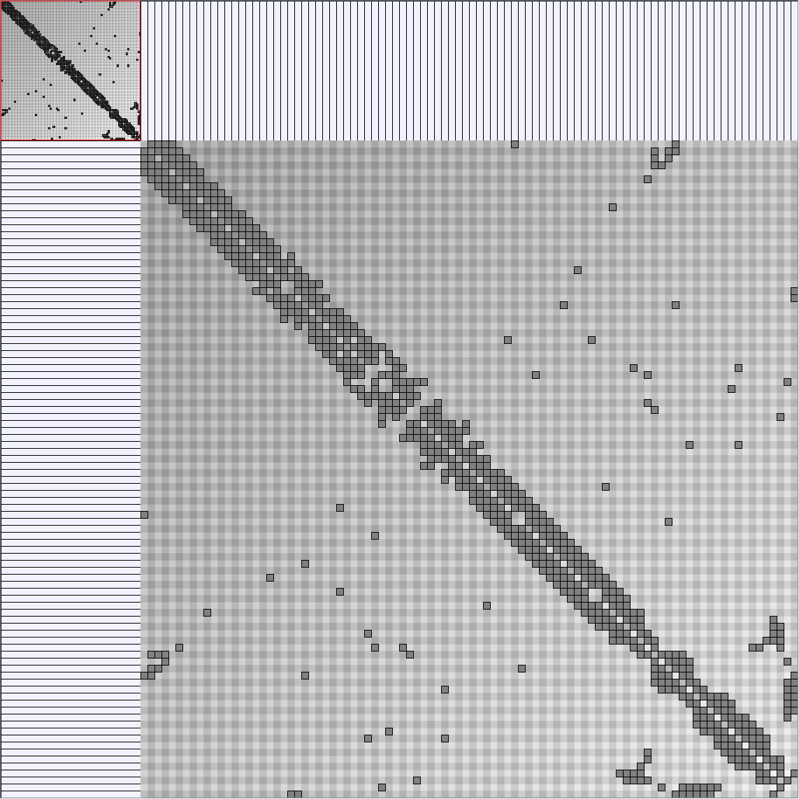
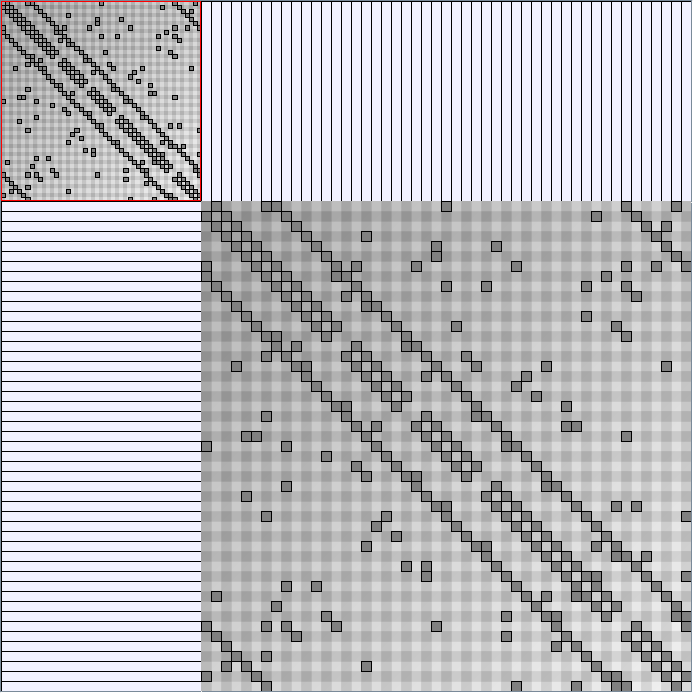
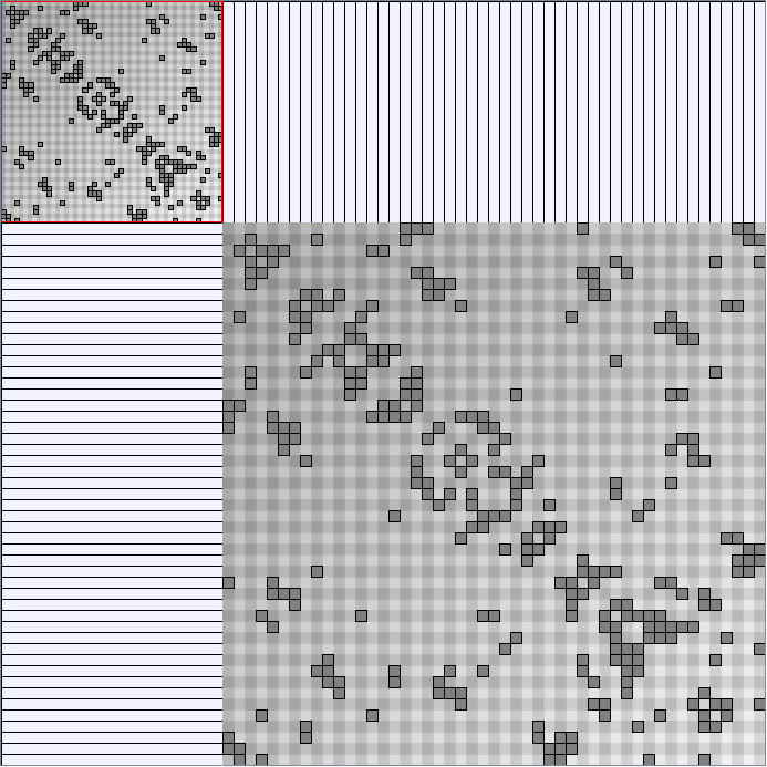
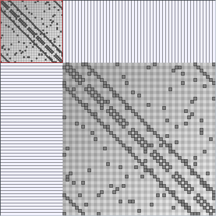
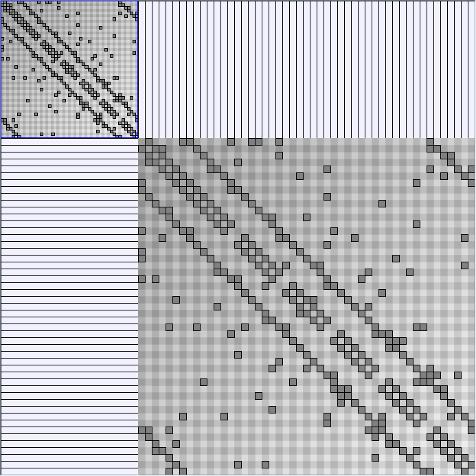
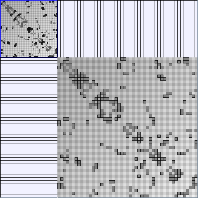
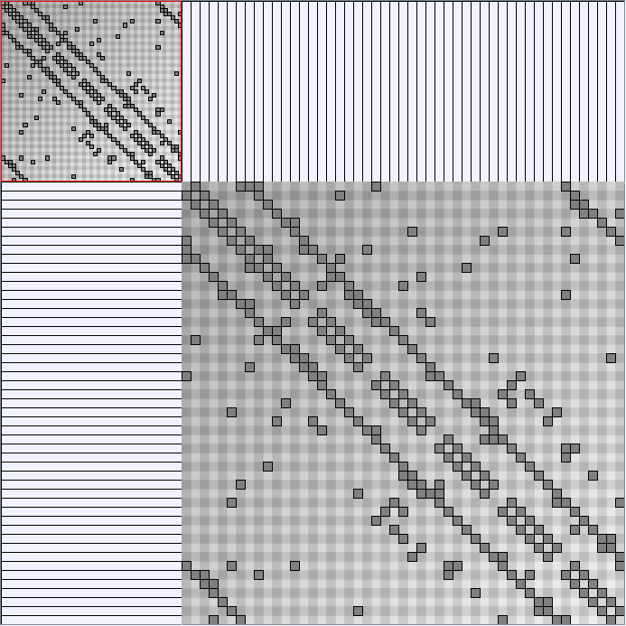
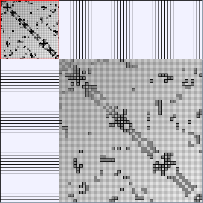
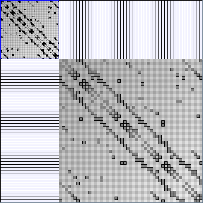
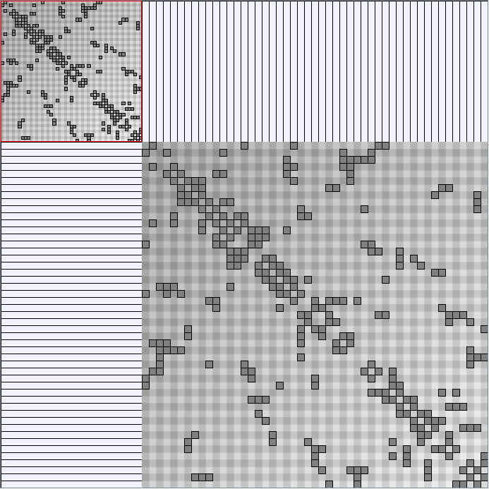
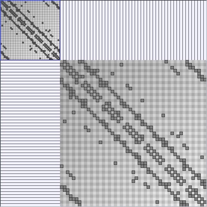
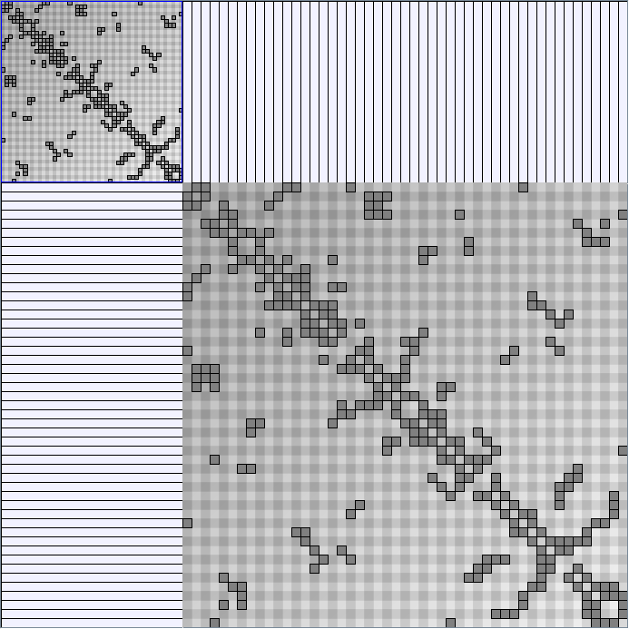
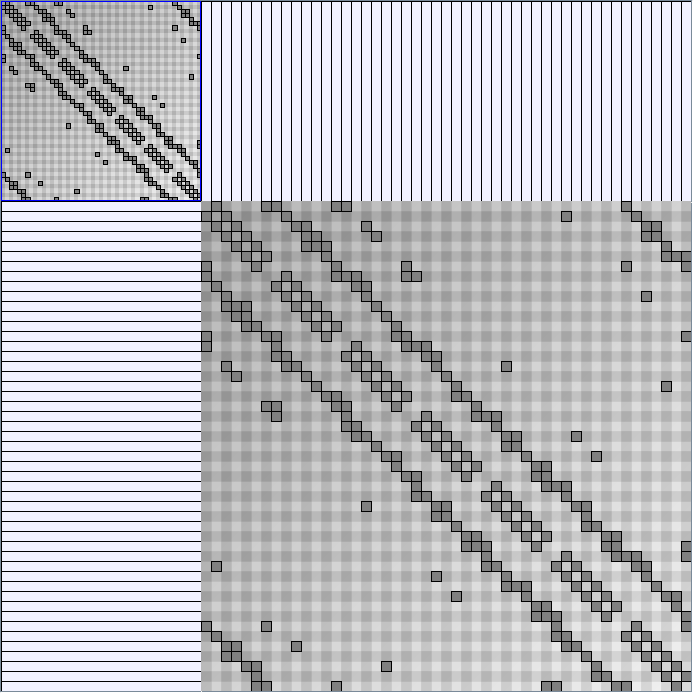
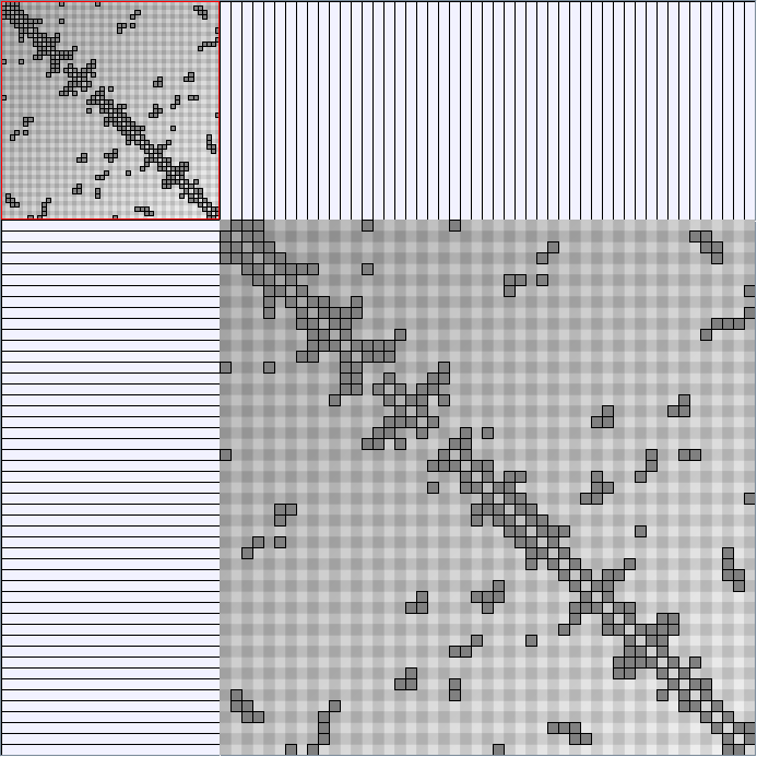
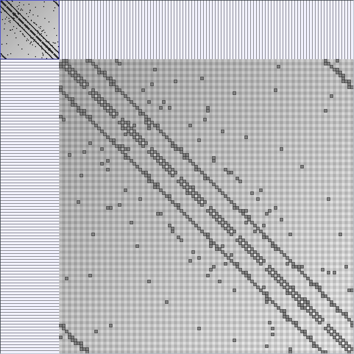
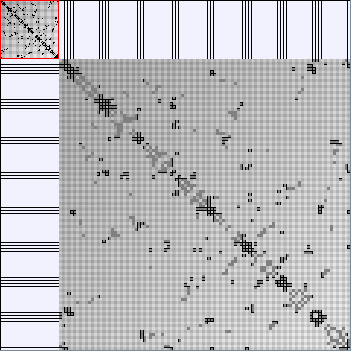
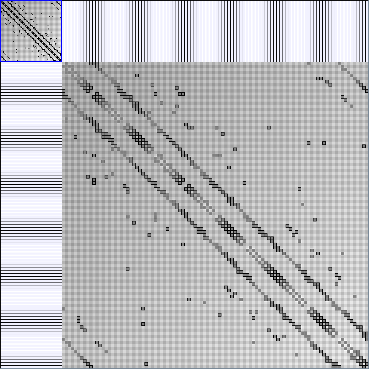
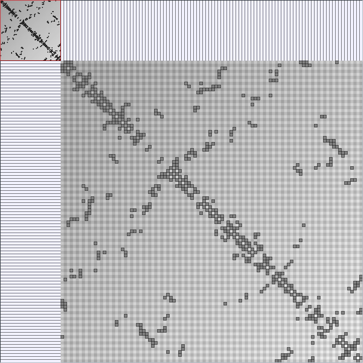
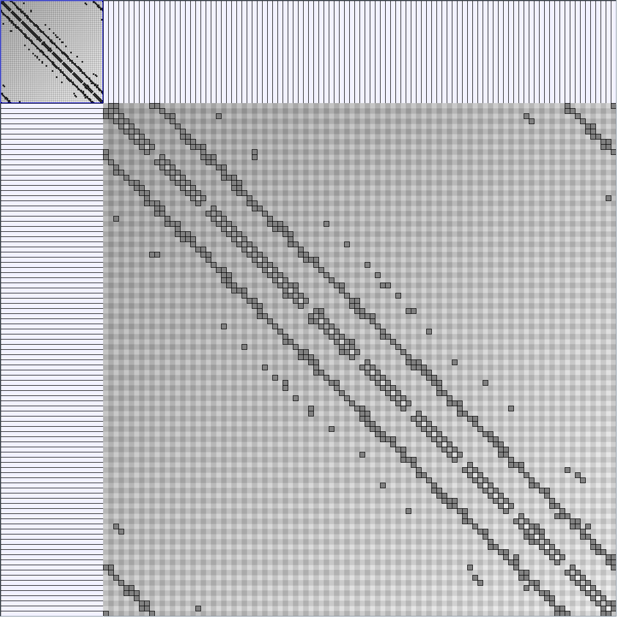
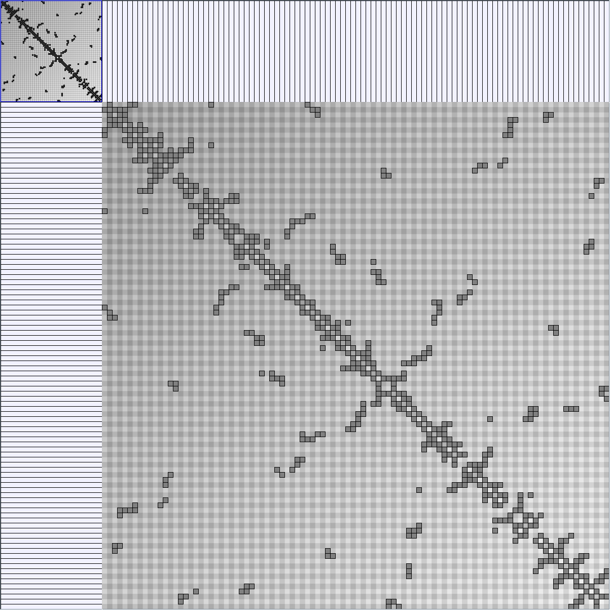
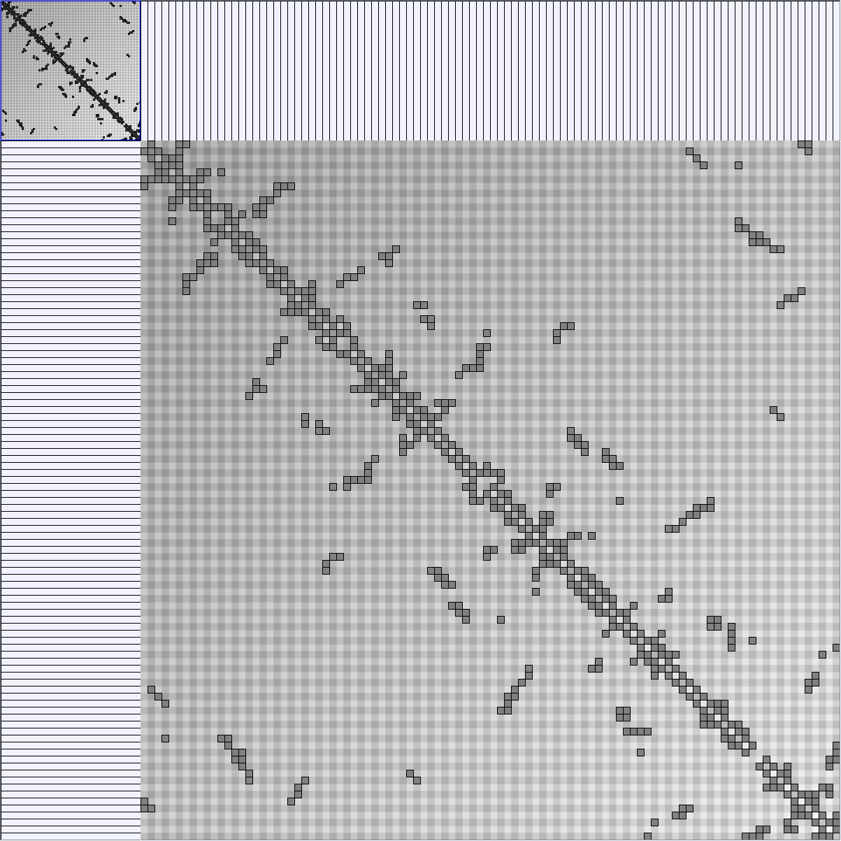
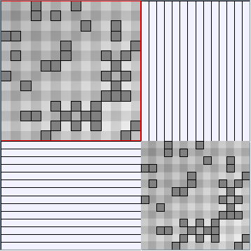
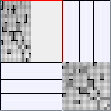
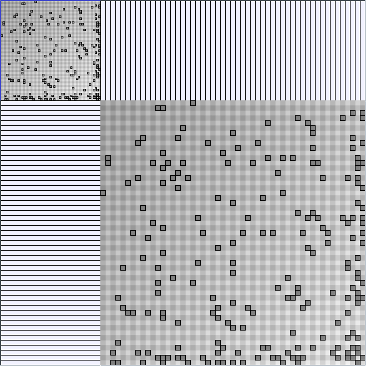
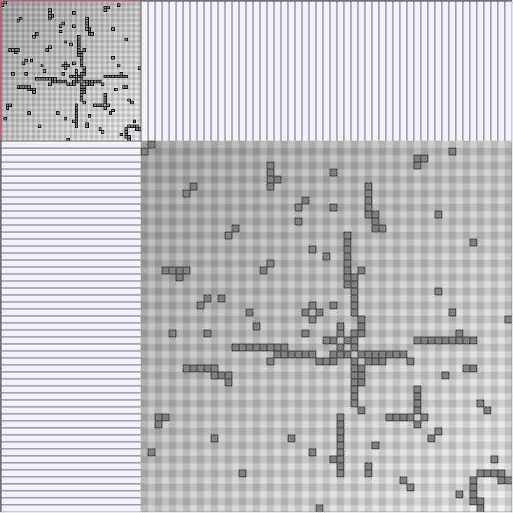
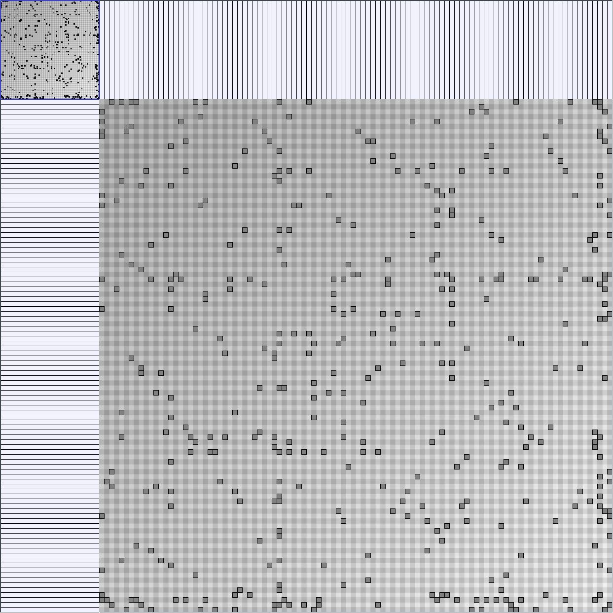
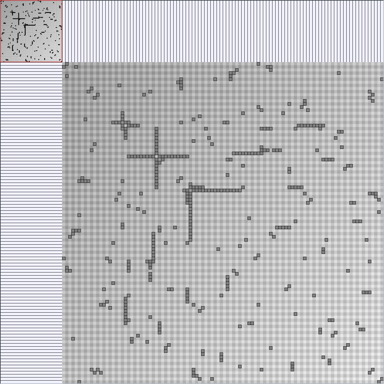
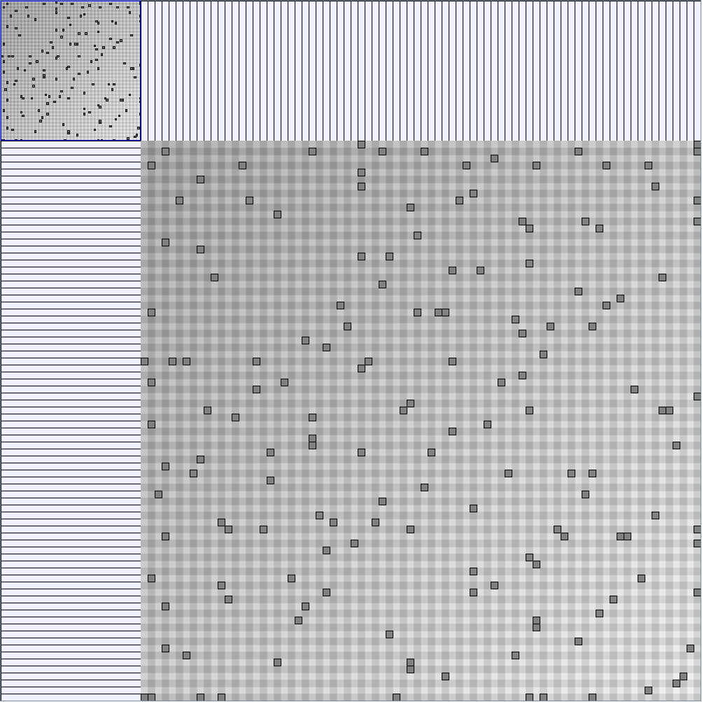
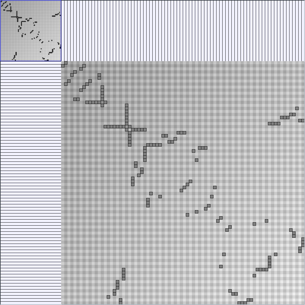
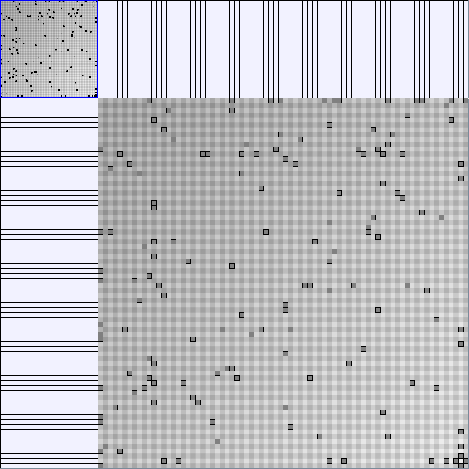
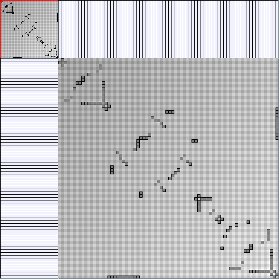
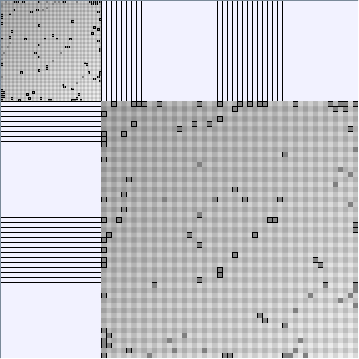
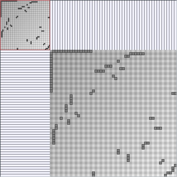
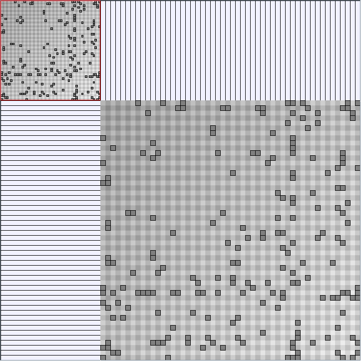
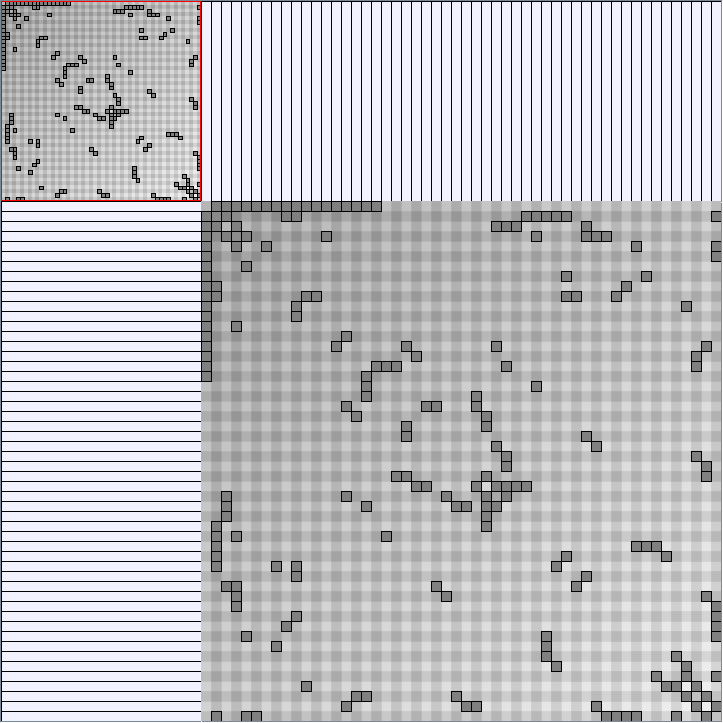
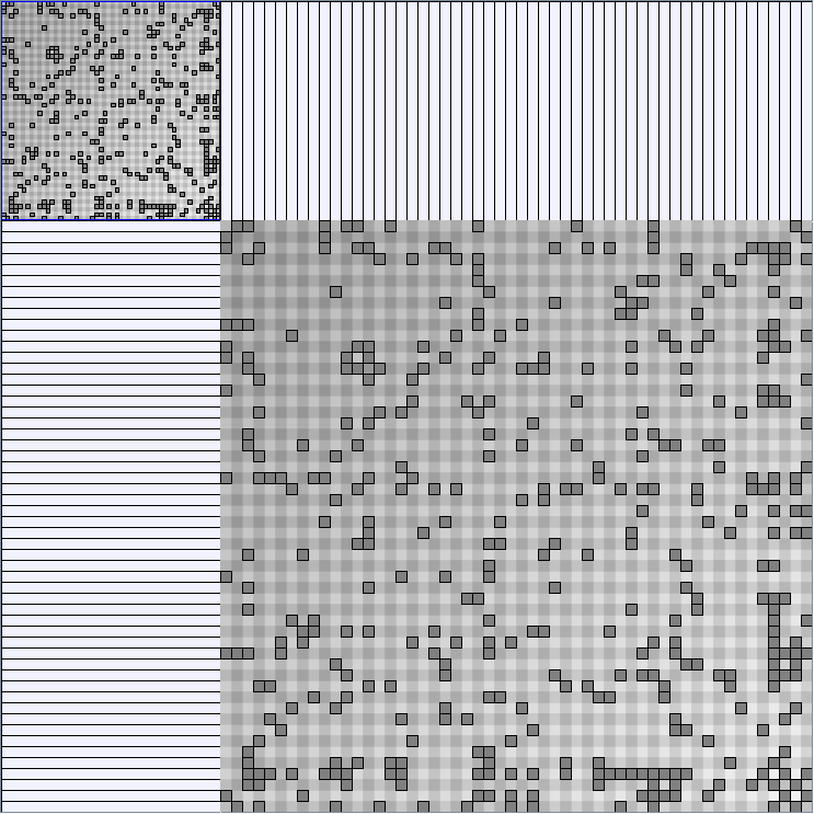
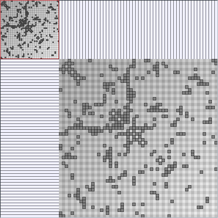
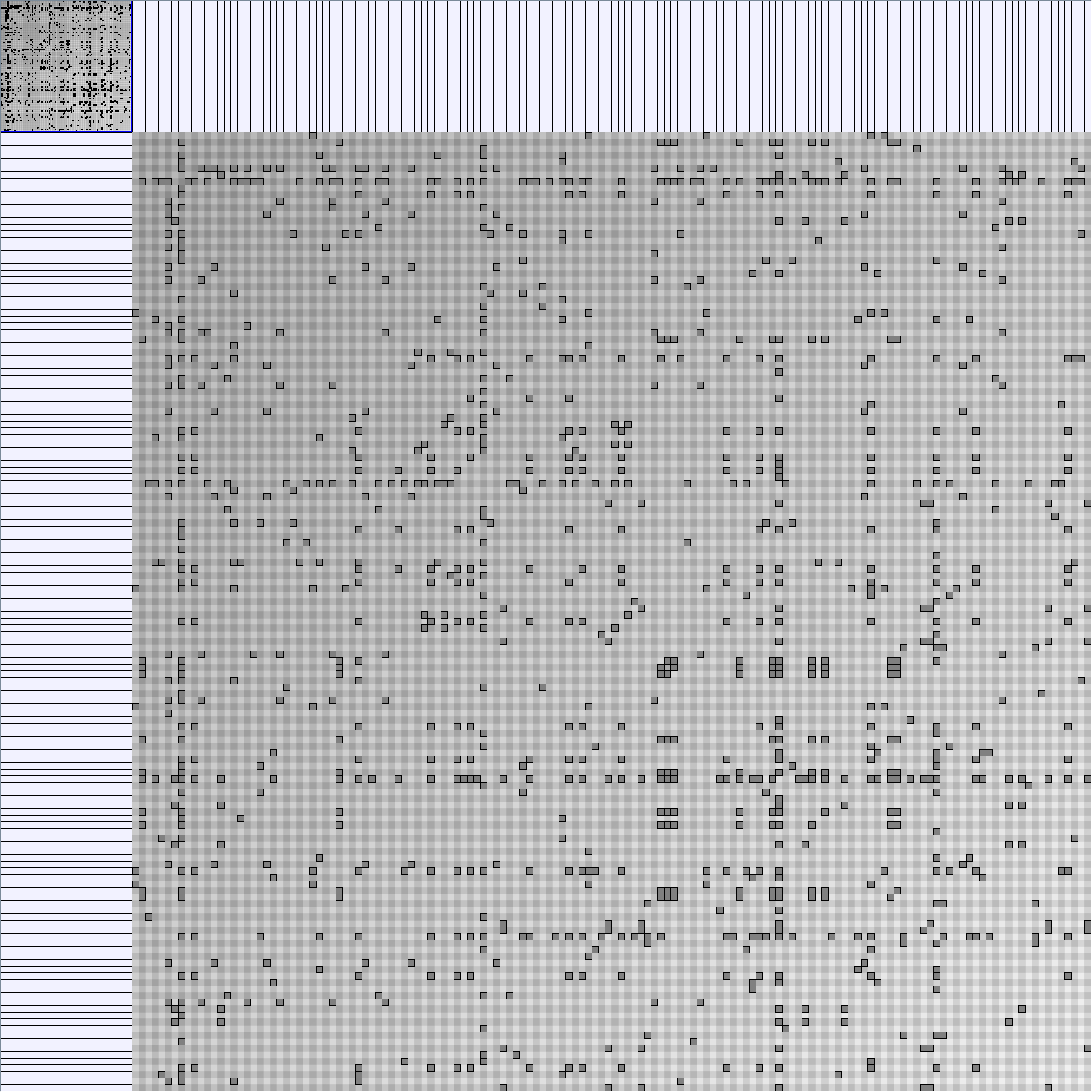
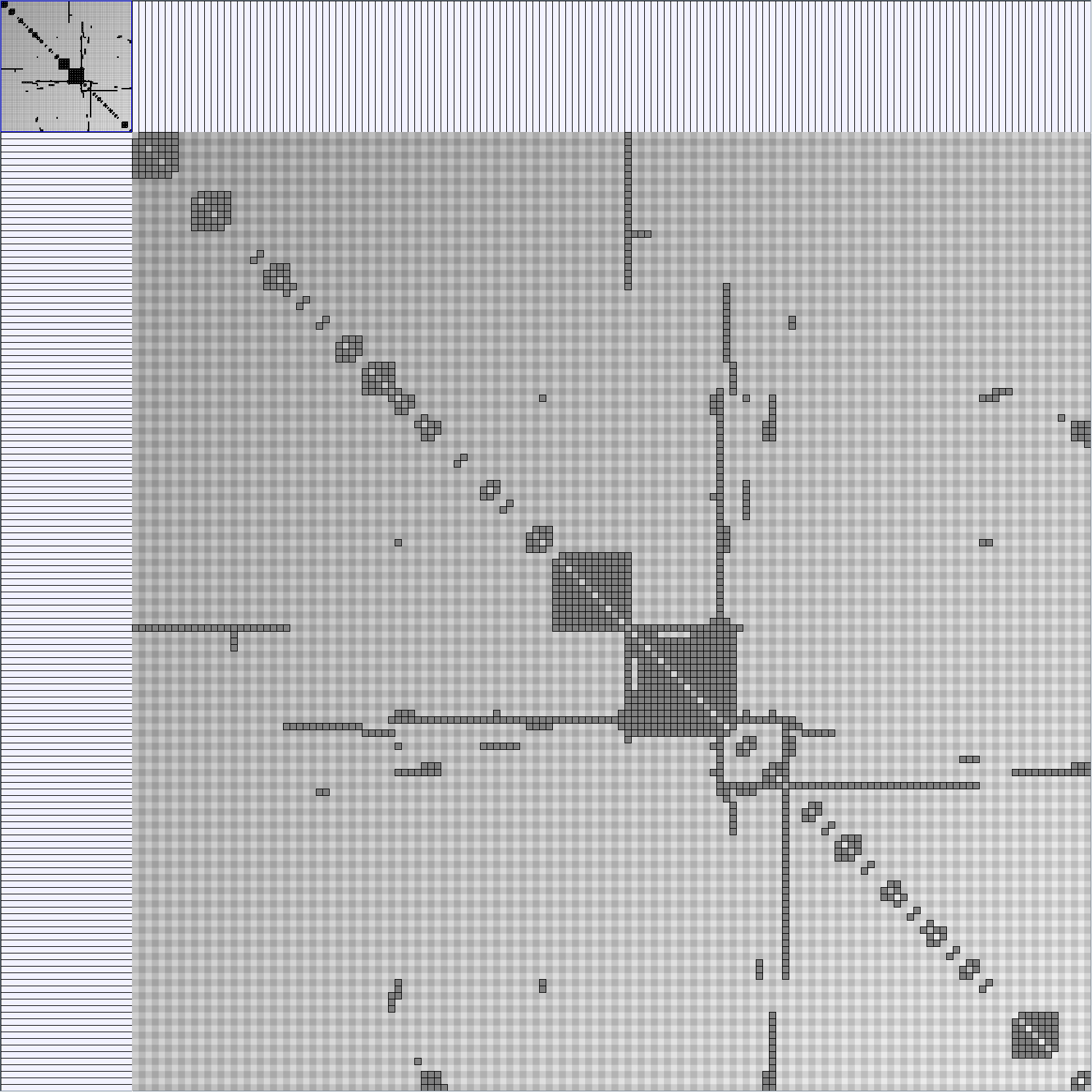
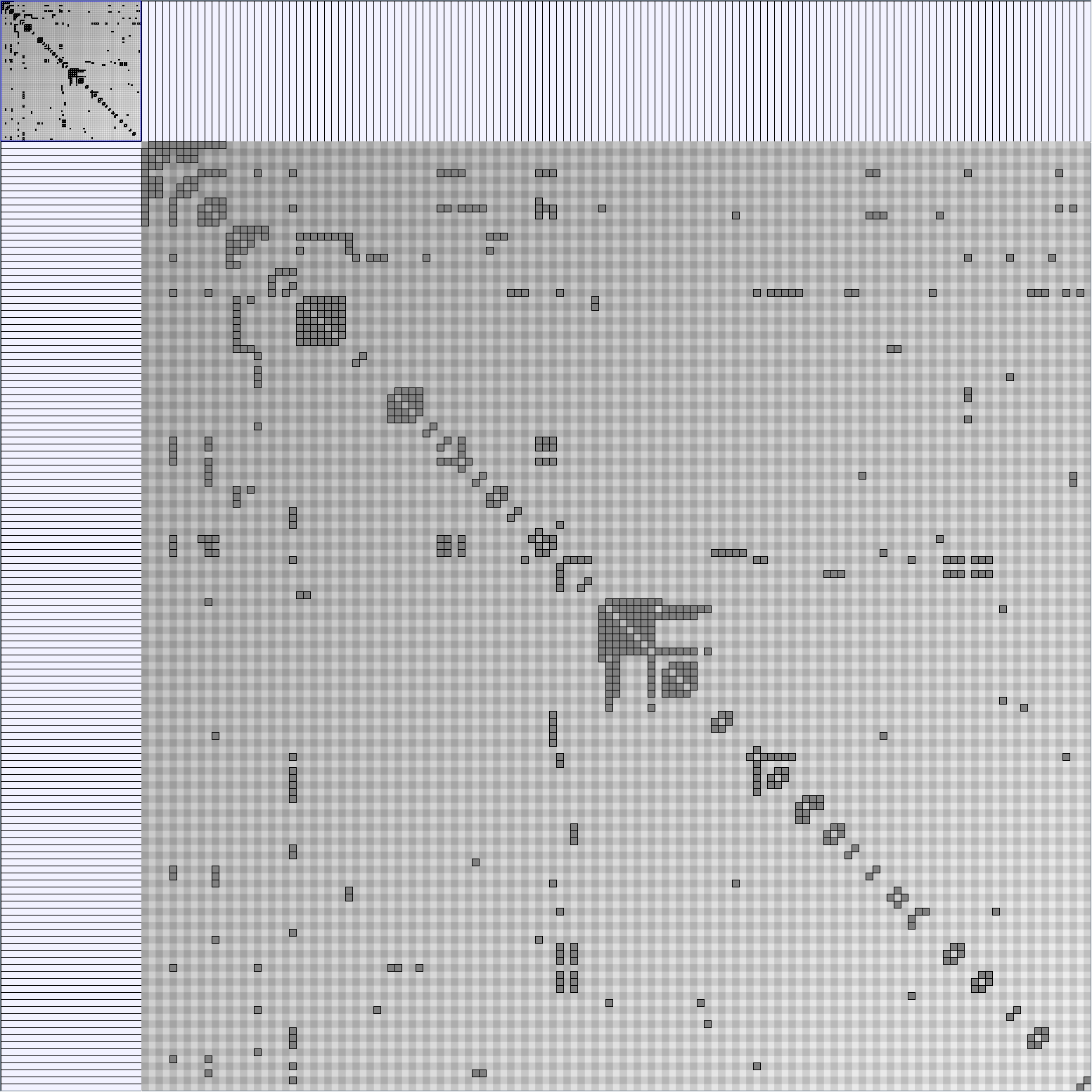
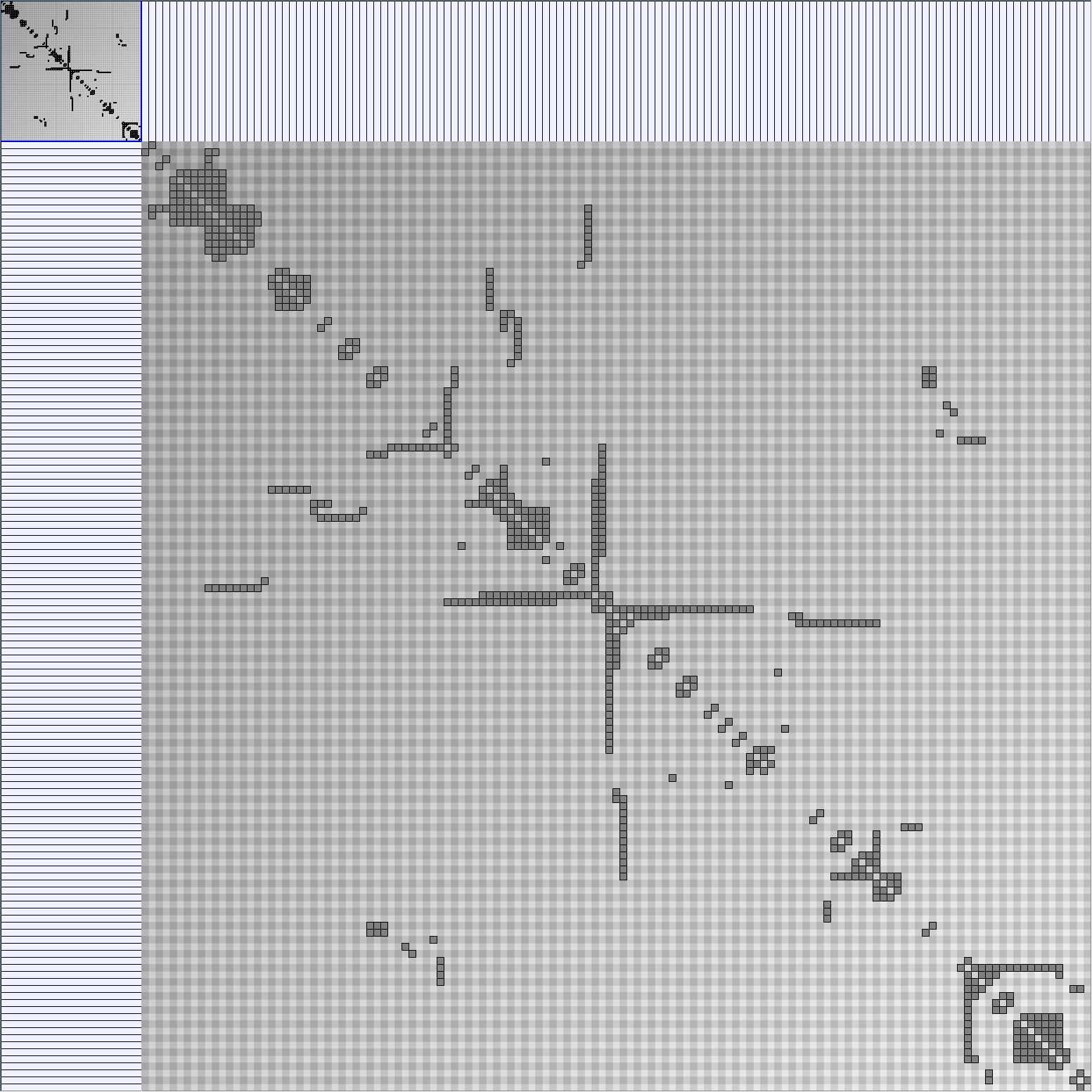
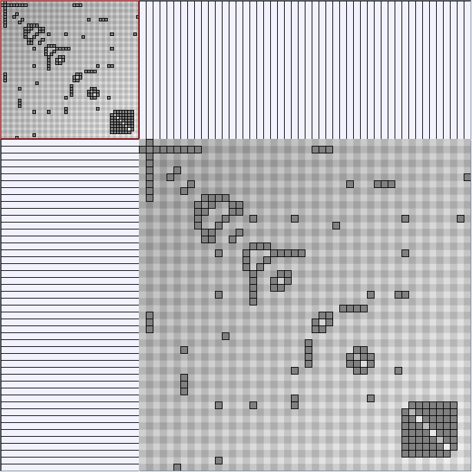
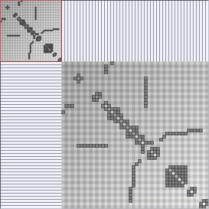
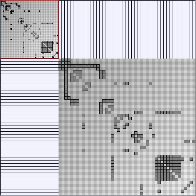
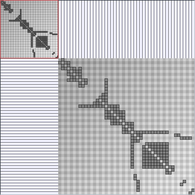
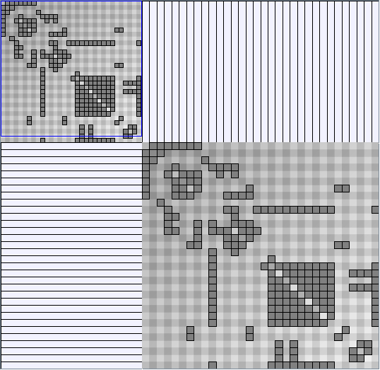
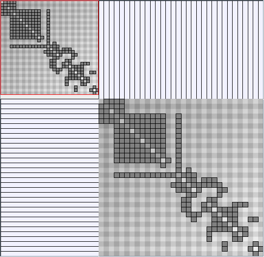
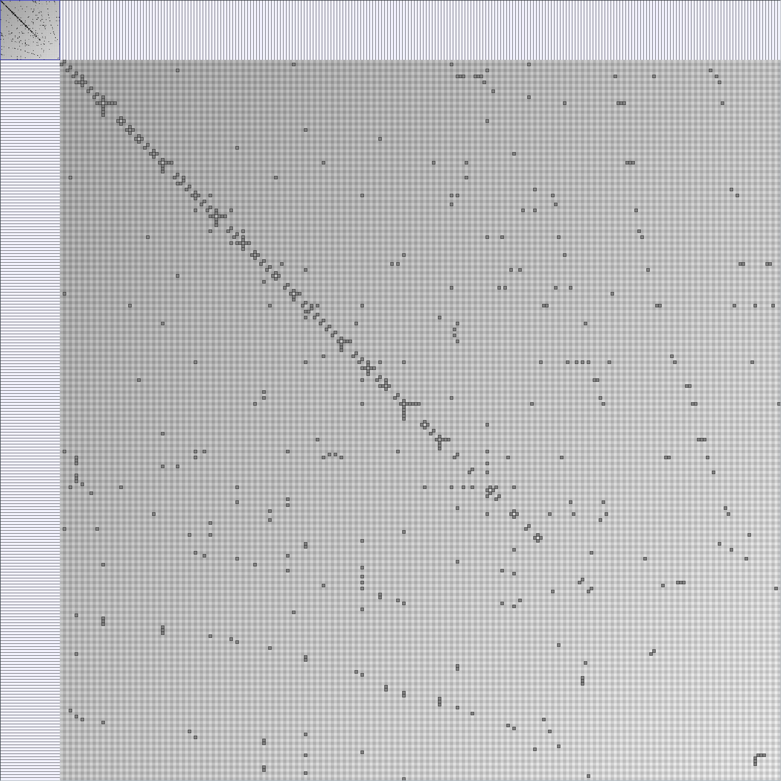
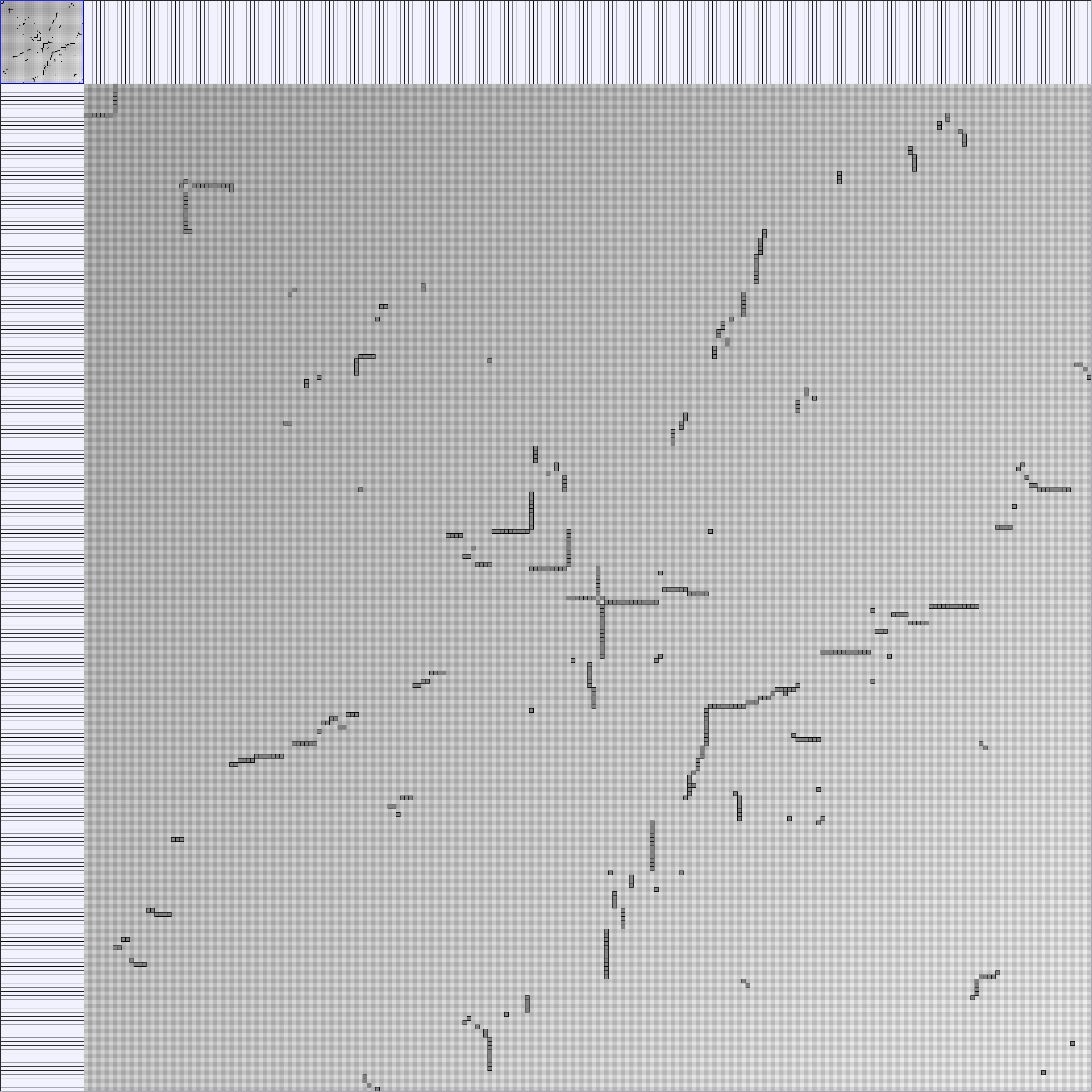
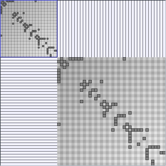
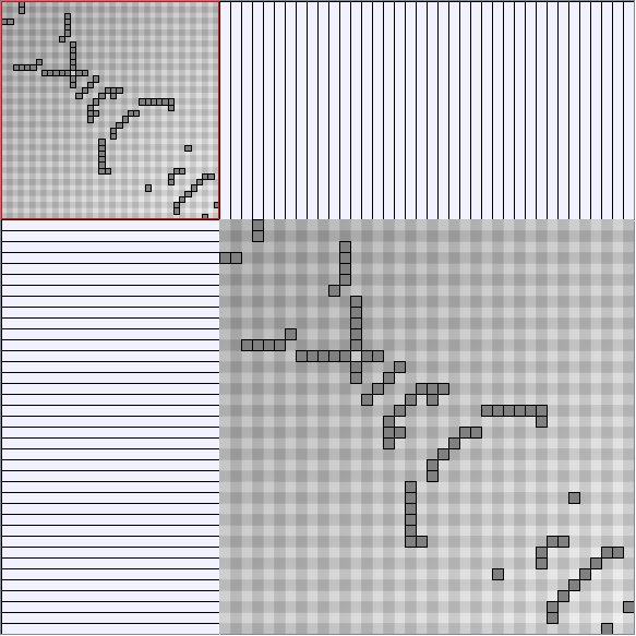
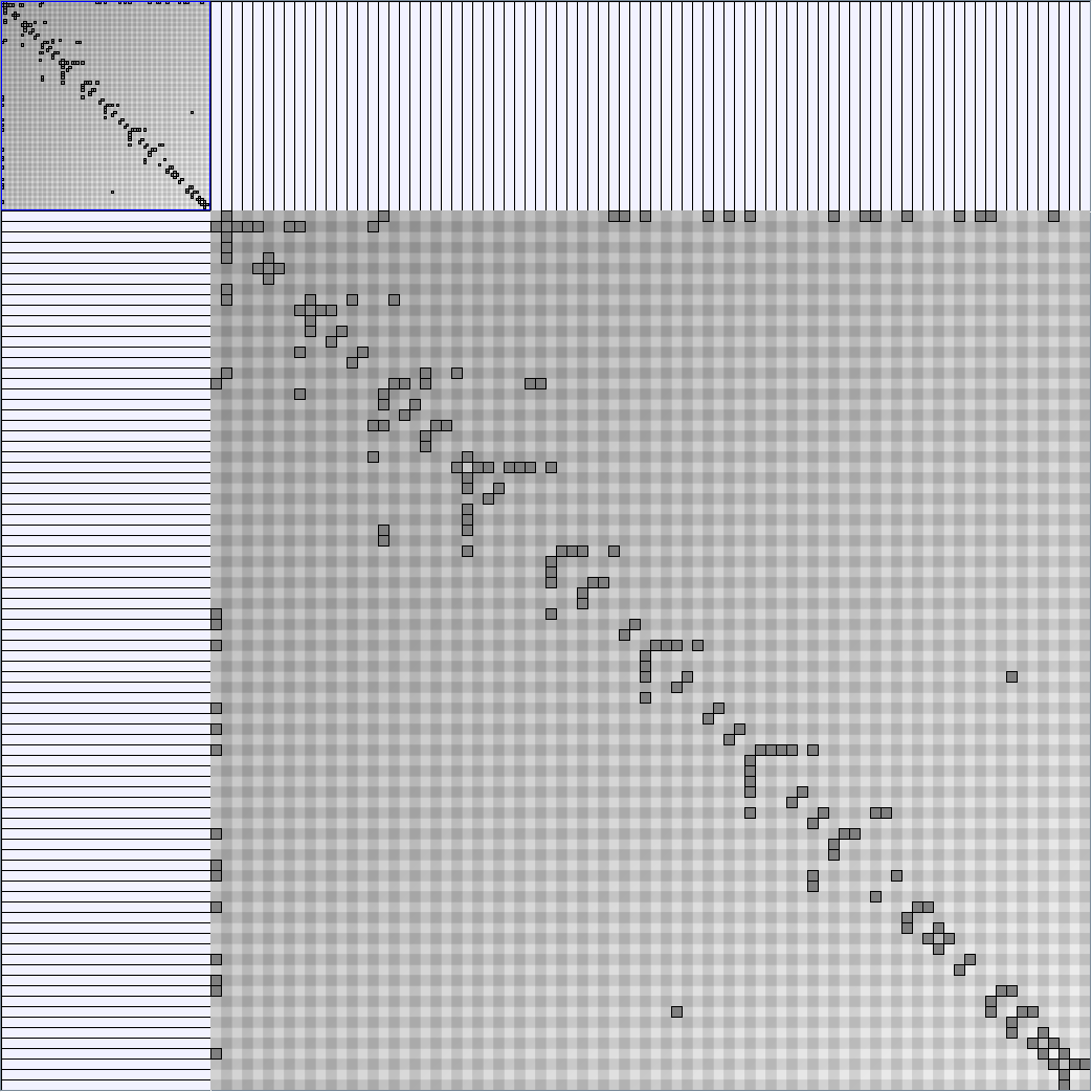
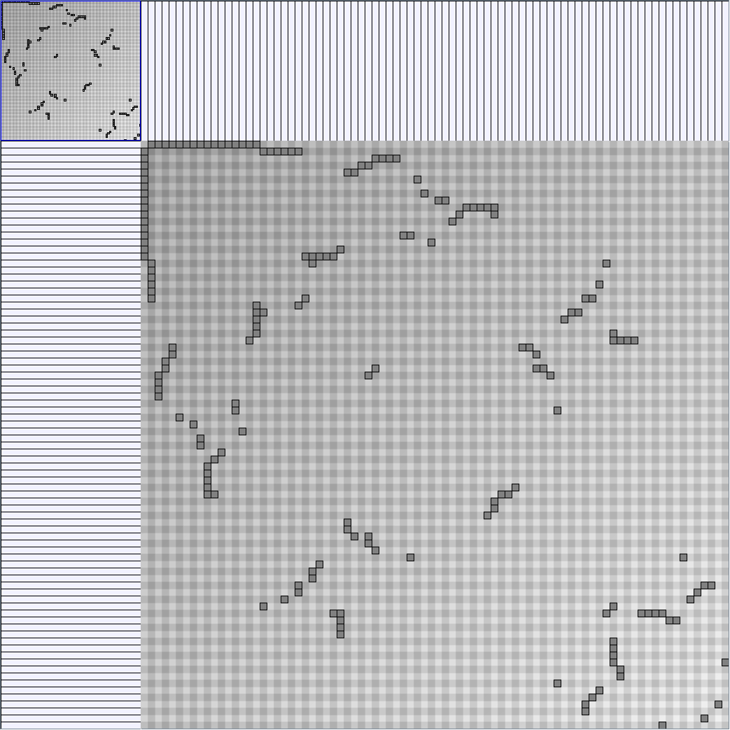
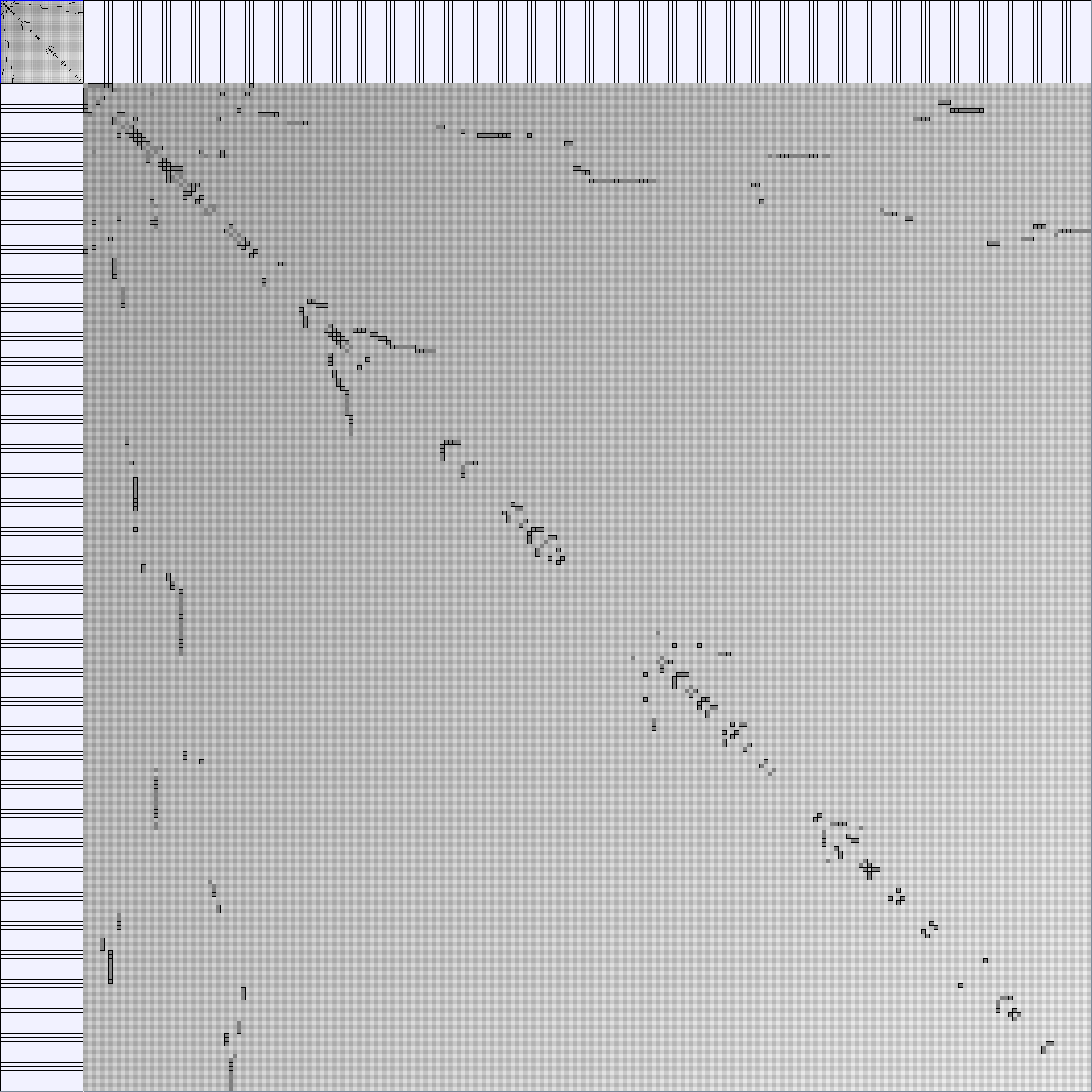
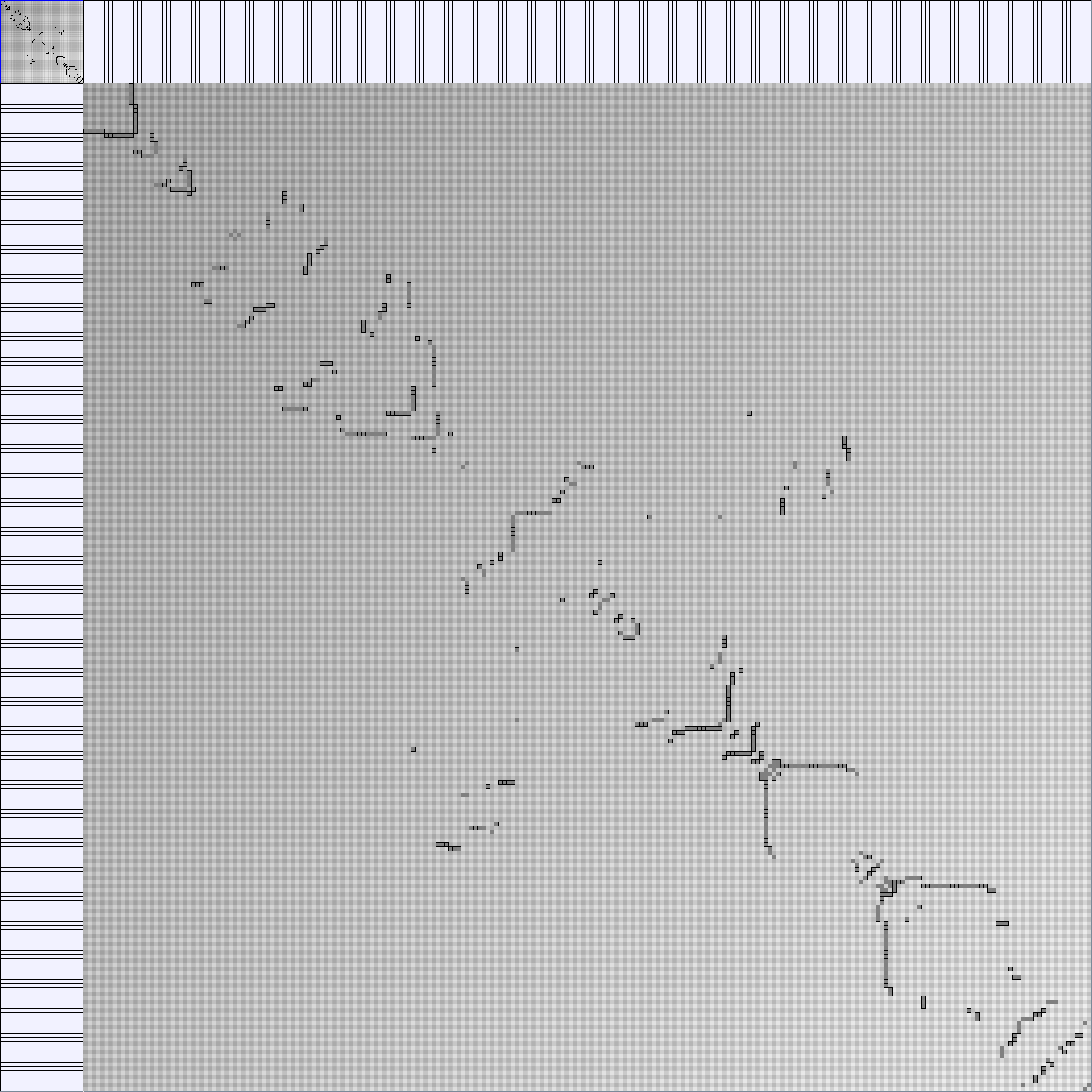
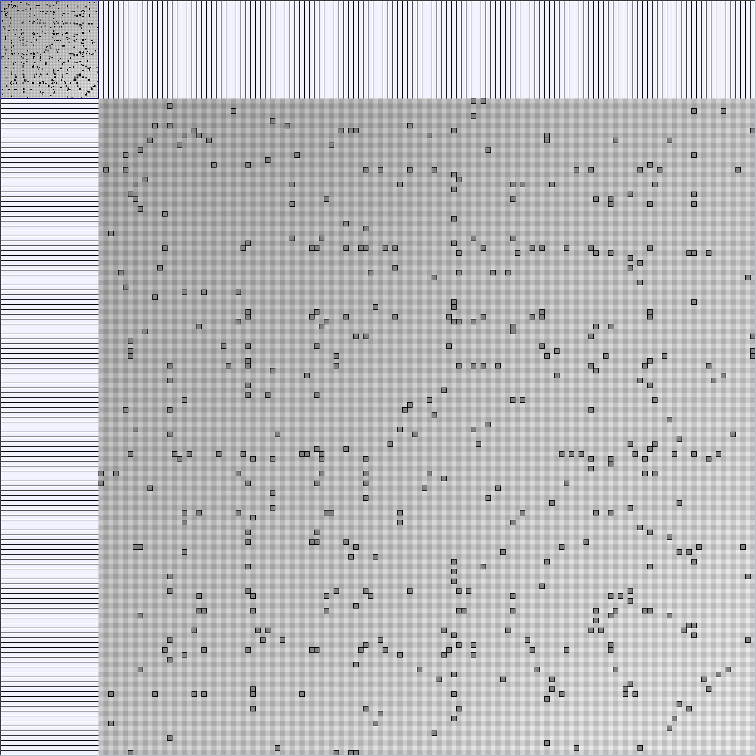
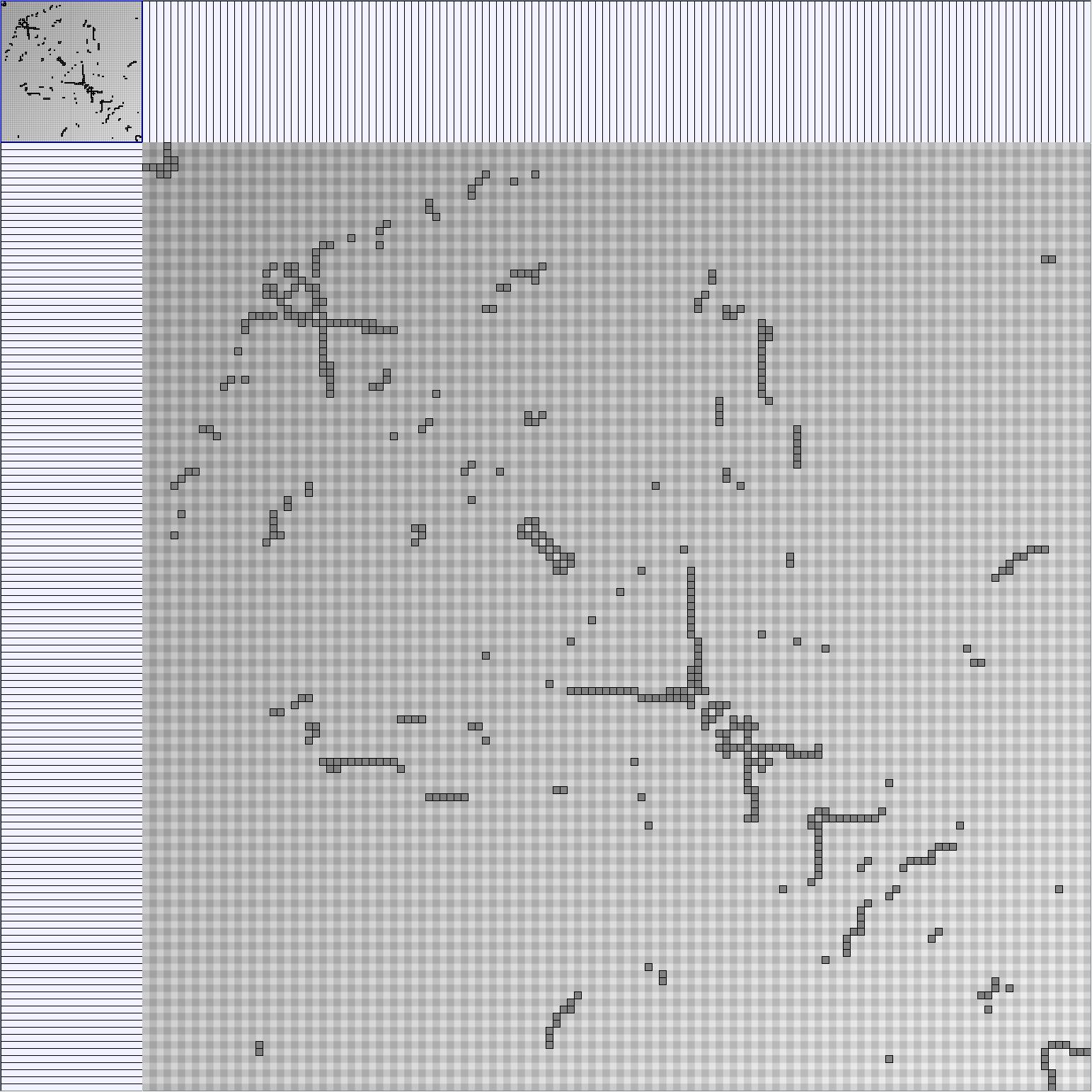
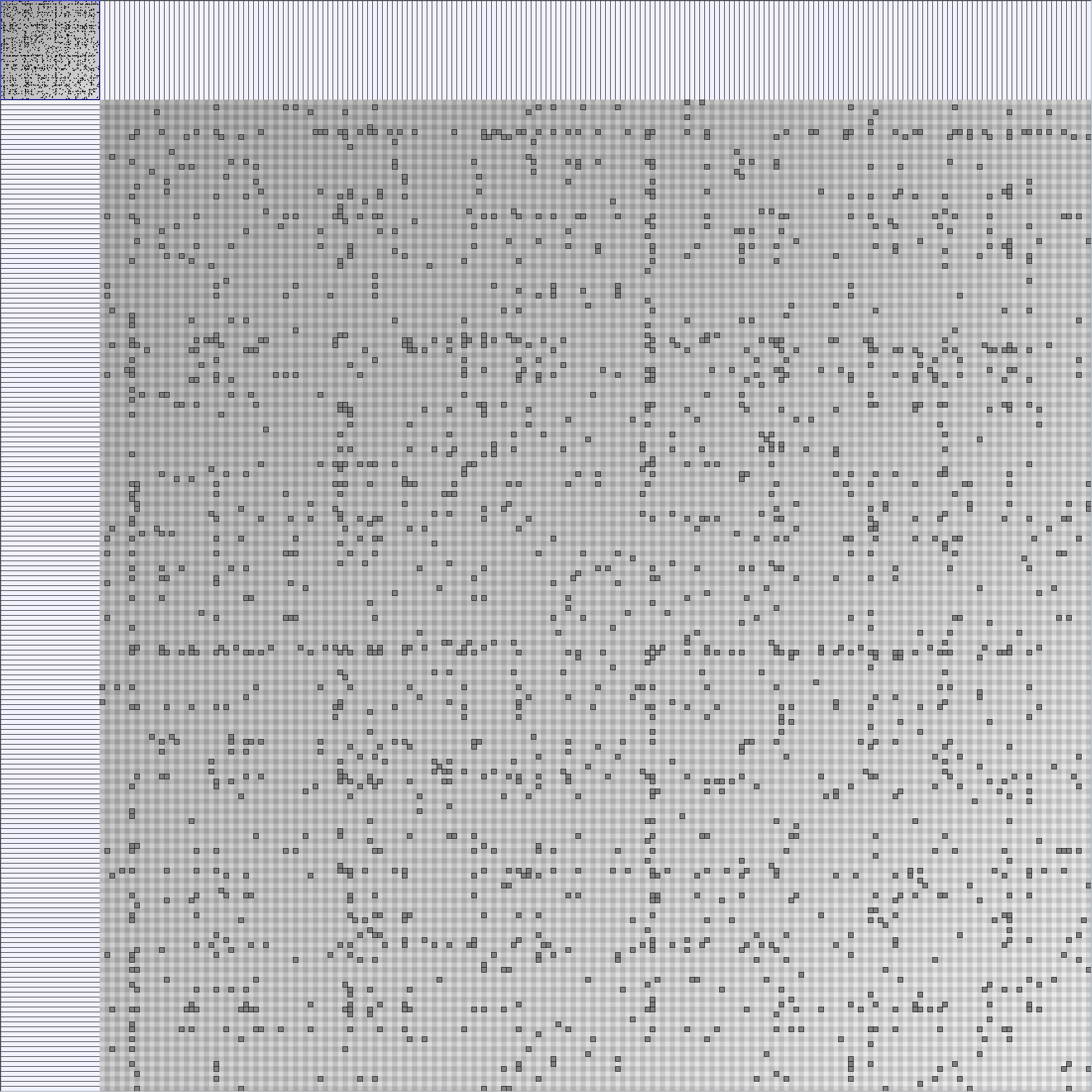
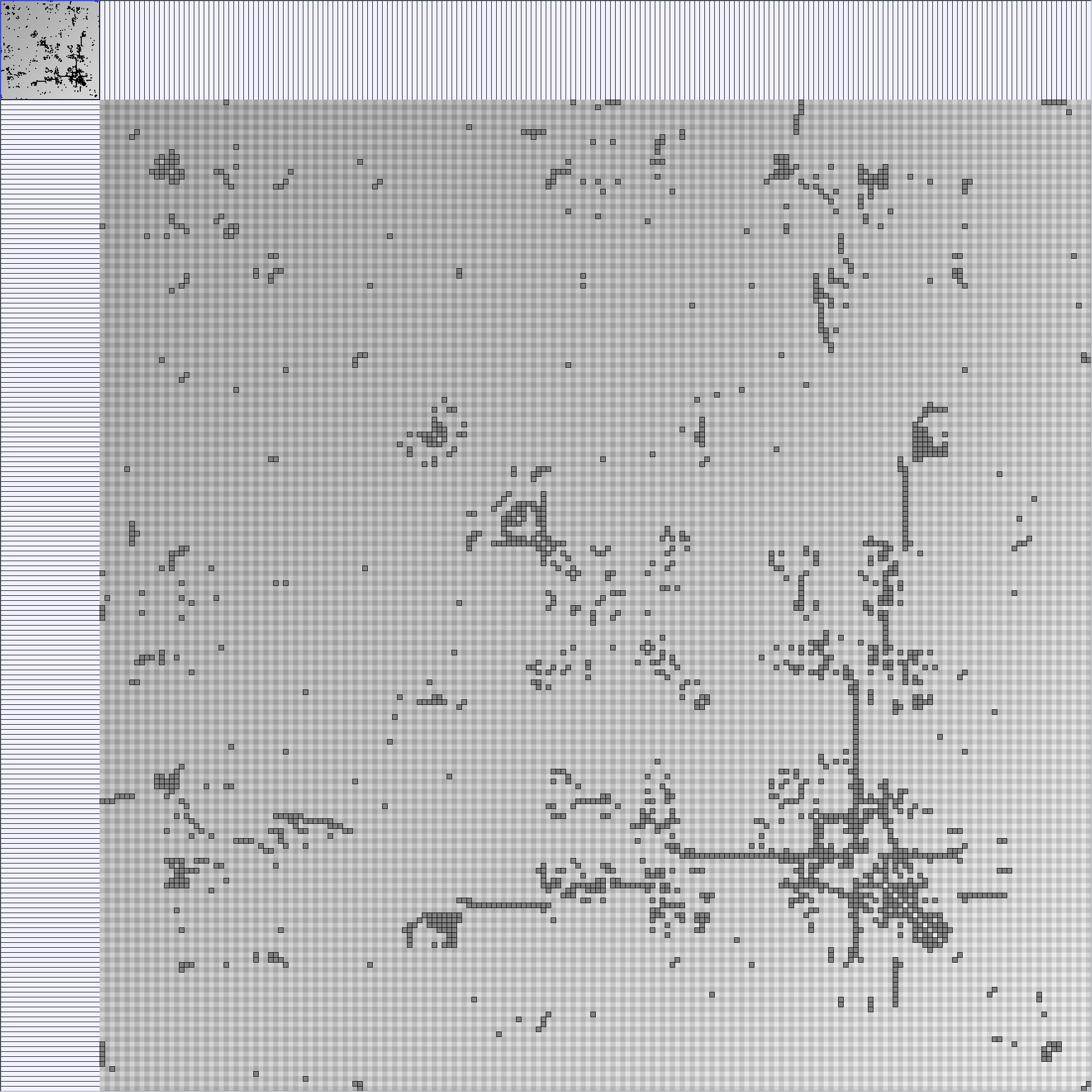
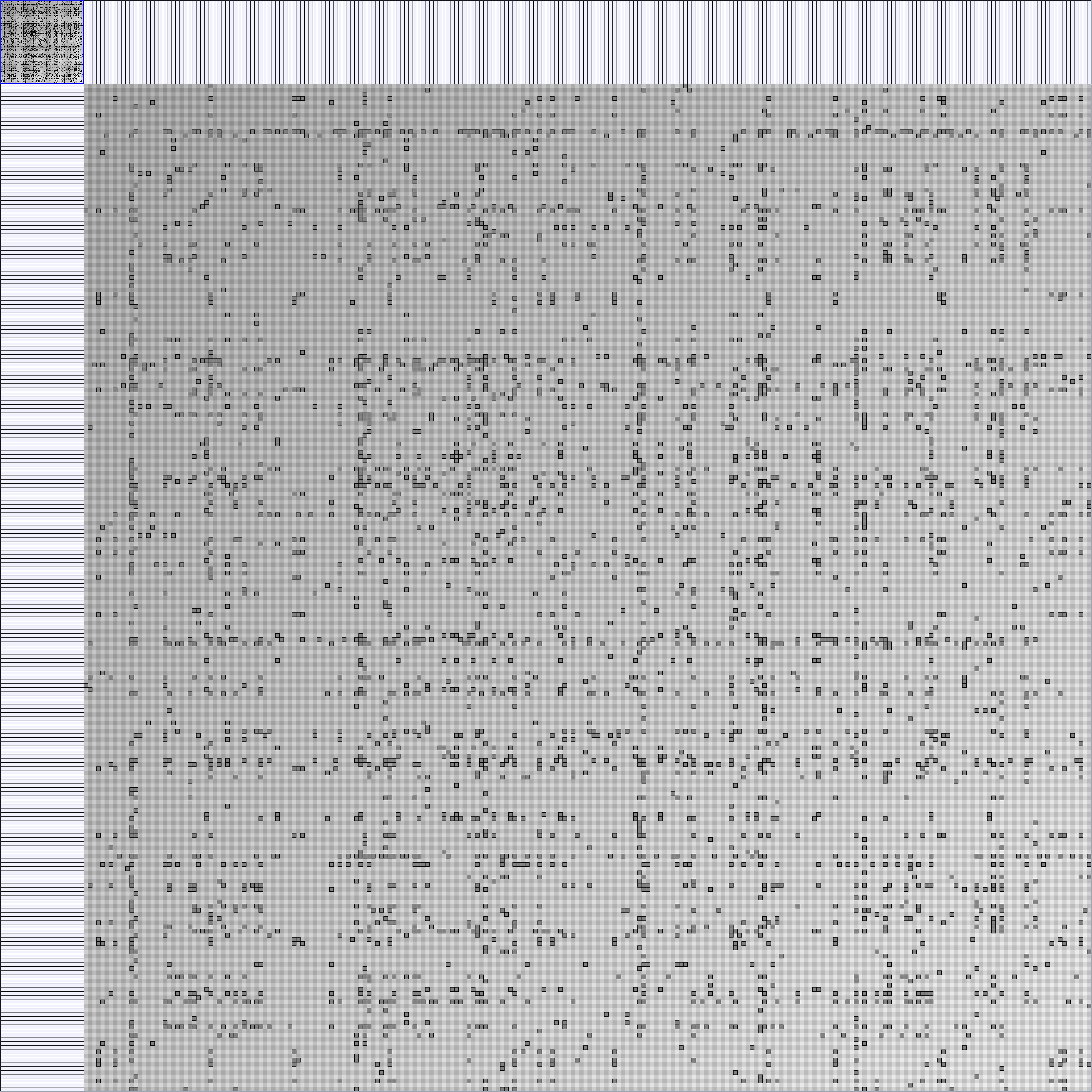
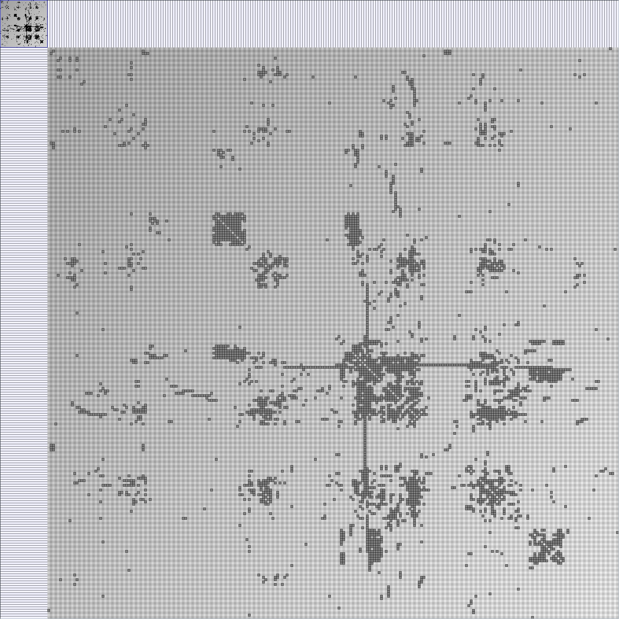
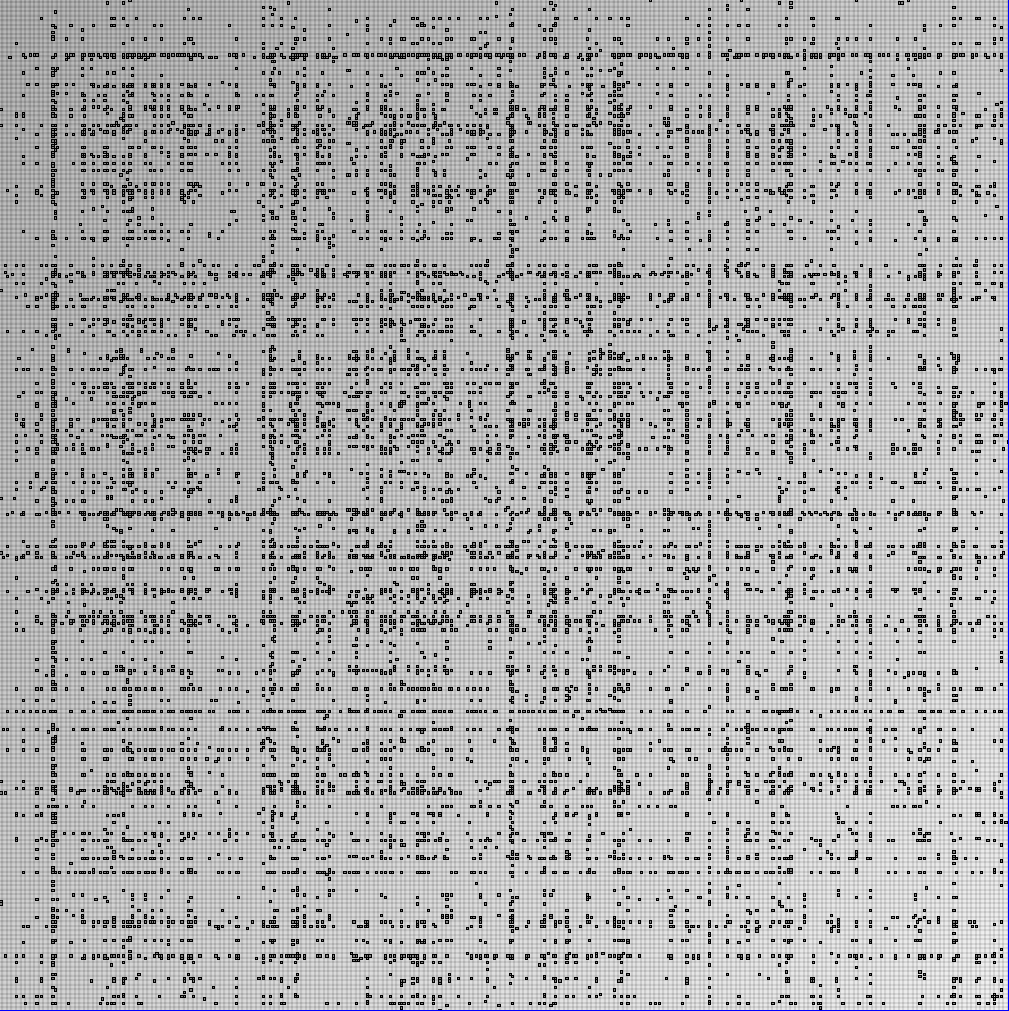
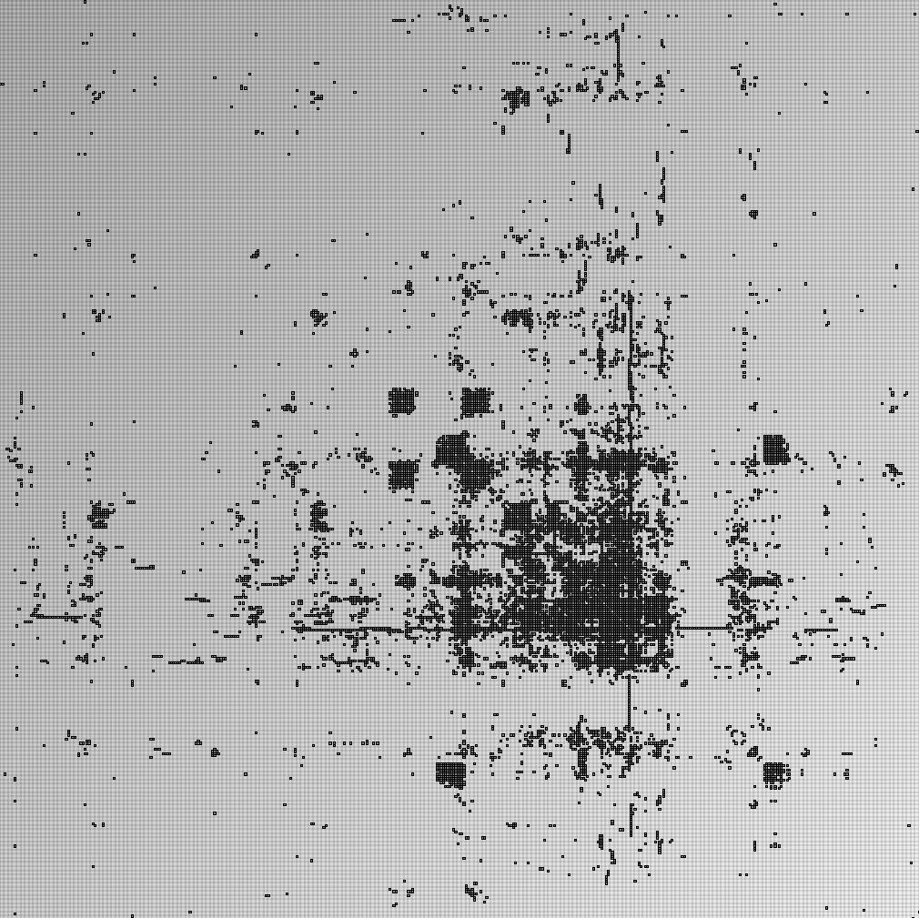
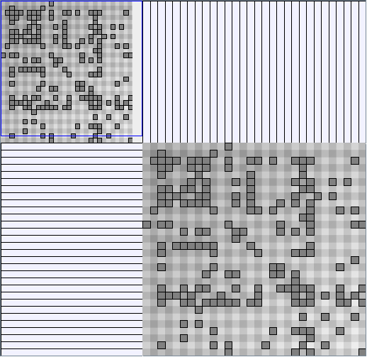
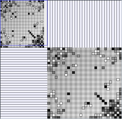
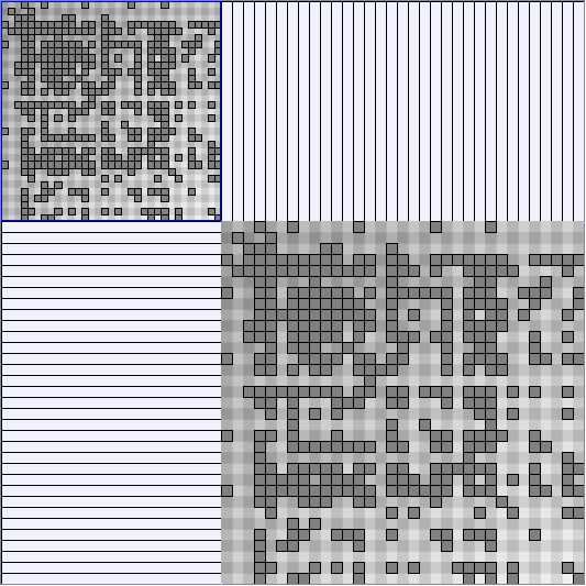
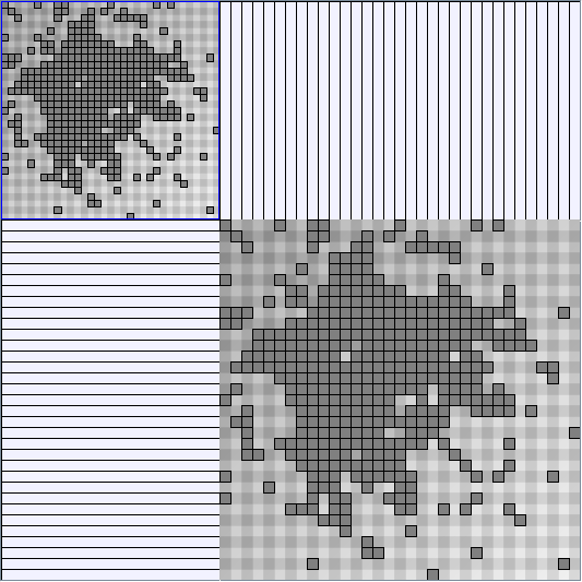
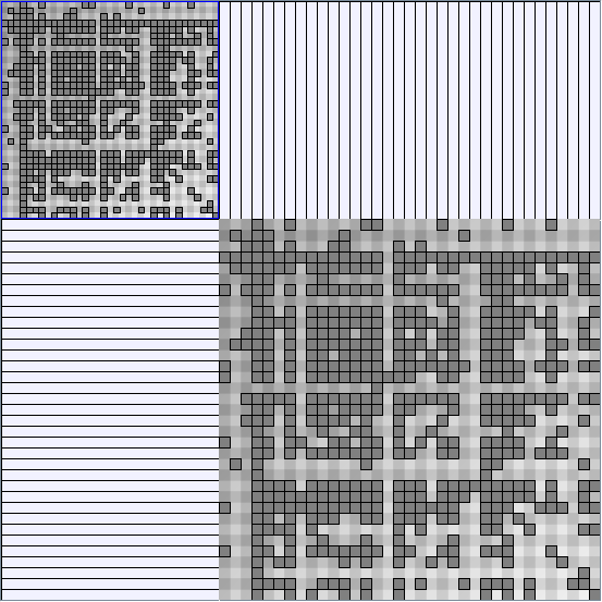
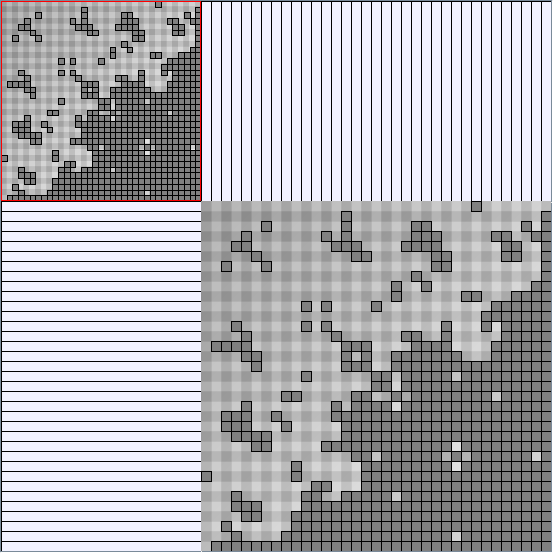
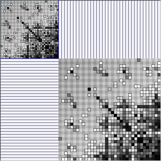
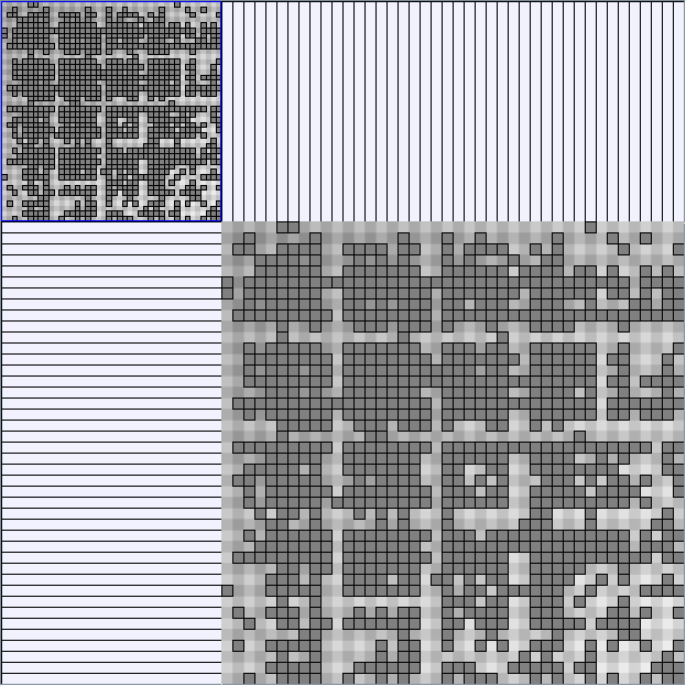
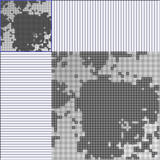
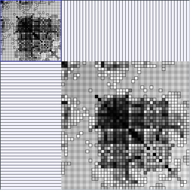
- Matrices are shown both with the initial order (middle image) and reordered with the TSP-Based algorithm (right image) described by Henry and Fekete [Infovis 2006].
Small-World Generators
WattsBetaSmallWorldGenerator
Parameters: numVertices (the number of nodes in the ring lattice), beta (the probability of an edge being rewired randomly; the proportion of randomly rewired edges in a graph) and degree( the number of edges connected to each vertex; the local neighborhood size). Degree must be even.
| Parameters and Resulting Graph characteristics | ||||||||||||
| graphs | W1 | W2 | W3 | W4 | W5 | W6 | W7 | W8 | W9 | W10 | W11 | W12 |
| numVertices | 47 | 47 | 47 | 47 | 47 | 47 | 47 | 47 | 47 | 47 | 47 | 94 |
| beta | 0.1 | 0.3 | 0.5 | 0.7 | 0.9 | 0.3 | 0.3 | 0.3 | 0.3 | 0.7 | 0.1 | 0.1 |
| degree | 6 | 6 | 6 | 6 | 6 | 2 | 4 | 8 | 10 | 4 | 8 | 8 |
| numVertices | 47 | 47 | 47 | 47 | 47 | 47 | 47 | 47 | 47 | 47 | 47 | 94 |
| numEdges | 282 | 282 | 282 | 282 | 282 | 94 | 188 | 376 | 470 | 188 | 376 | 752 |
| components | 1 | 1 | 1 | 1 | 1 | 2 | 1 | 1 | 1 | 1 | 1 | 1 |
| density | 0.36 | 0.36 | 0.36 | 0.36 | 0.36 | 0.21 | 0.29 | 0.41 | 0.46 | 0.29 | 0.41 | 0.29 |
| clusteringCoefficient | 0.51 | 0.25 | 0.15 | 0.09 | 0.12 | 0.23 | 0.25 | 0.32 | 0.38 | 0.07 | 0.53 | 0.52 |
| diameter | 6 | 4 | 4 | 4 | 4 | - | 6 | 4 | 3 | 5 | 5 | 6 |
| averageShortestDistance | 2.97 | 2.4 | 2.32 | 2.3 | 2.29 | - | 3.24 | 2.15 | 1.98 | 2.83 | 2.56 | 3.15 |
| minDegree | 5 | 4 | 4 | 3 | 4 | 1 | 2 | 5 | 8 | 2 | 7 | 6 |
| maxDegree | 8 | 9 | 9 | 9 | 9 | 4 | 6 | 10 | 13 | 8 | 10 | 10 |
KleinbergSmallWorldGenerator
Parameters:latticeSize (the lattice size (length of row or column dimension)) and clusteringExponent (the clustering exponent parameter).
| Parameters and Resulting Graph characteristics | |||||||||||
| graphs | W1 | W2 | W3 | W4 | W5 | W6 | W7 | W8 | W9 | W10 | W11 |
| latticeSize | 7 | 7 | 7 | 7 | 7 | 7 | 7 | 10 | 10 | 10 | 10 |
| clusteringExponent | 0.1 | 0.5 | 1 | 2 | 2.5 | 4 | 8 | 2 | 4 | 8 | 12 |
| numVertices | 49 | 49 | 49 | 49 | 49 | 49 | 49 | 100 | 100 | 100 | 100 |
| numEdges | 490 | 490 | 490 | 490 | 490 | 490 | 490 | 1000 | 1000 | 1000 | 1000 |
| components | 1 | 1 | 1 | 1 | 1 | 1 | 1 | 1 | 1 | 1 | 1 |
| density | 0.45 | 0.45 | 0.45 | 0.45 | 0.45 | 0.45 | 0.45 | 0.32 | 0.32 | 0.32 | 0.32 |
| clusteringCoefficient | 0.08 | 0.09 | 0.14 | 0.19 | 0.19 | 0.26 | 0.32 | 0.18 | 0.23 | 0.32 | 0.33 |
| diameter | 4 | 4 | 4 | 4 | 4 | 5 | 5 | 5 | 6 | 7 | 7 |
| averageShortestDistance | 2.38 | 2.36 | 2.37 | 2.44 | 2.48 | 2.54 | 2.73 | 3.1 | 3.57 | 3.65 | 3.68 |
| minDegree | 9 | 9 | 9 | 9 | 9 | 9 | 9 | 9 | 9 | 9 | 9 |
| maxDegree | 14 | 12 | 13 | 12 | 12 | 13 | 12 | 13 | 13 | 14 | 12 |
Scale-Free Networks Generator
BarabasiAlbertGenerator
Parameters: init_vertices (number of vertices that the graph should start with), numEdgesToAttach (the number of edges that should be attached from the new vertex to pre-existing vertices at each time step) and numSteps (number of time steps). init_vertices must be superior or equal to numEdgesToAttach.
| Parameters and Resulting Graph characteristics | ||||||||
| graphs | W1 | W2 | W3 | W4 | W5 | W6 | W7 | W8 |
| init_vertices | 4 | 4 | 4 | 4 | 2 | 2 | 2 | 4 |
| numEdgesToAttach | 2 | 2 | 2 | 1 | 1 | 1 | 2 | 4 |
| numSteps | 10 | 50 | 100 | 100 | 100 | 50 | 50 | 50 |
| numVertices | 14 | 53 | 104 | 80 | 76 | 51 | 52 | 54 |
| numEdges | 40 | 200 | 400 | 158 | 150 | 100 | 200 | 400 |
| components | 1 | 1 | 1 | 1 | 1 | 1 | 1 | 1 |
| density | 0.45 | 0.27 | 0.19 | 0.16 | 0.16 | 0.2 | 0.27 | 0.37 |
| clusteringCoefficient | 0.15 | 0.2 | 0.07 | 0.51 | 0.51 | 0.66 | 0.16 | 0.23 |
| diameter | 4 | 6 | 6 | 11 | 14 | 8 | 5 | 4 |
| averageShortestDistance | 2.24 | 2.81 | 3.18 | 5.26 | 5.7 | 3.74 | 2.8 | 2.15 |
| minDegree | 2 | 1 | 2 | 1 | 1 | 1 | 2 | 4 |
| maxDegree | 5 | 16 | 19 | 8 | 12 | 16 | 17 | 26 |
EppsteinPowerLawGenerator
Parameters: numVertices (the number of vertices for the generated graph), numEdges (the number of edges the generated graph will have, should be Theta(numVertices)) and r (the model parameter).
Real Social Networks
Here is a panel of undirected networks issued from scientific articles, benchmarks or contests. Social network visualization or analysis tools provide also some real datasets: Pajek [3] and UCINet [4].
Small-World
| Parameters and Resulting Graph characteristics for Co-Authoring Networks | Name | Team Collaboration (with external collaborators) | Infovis component 1 | Infovis component 2 | Infovis component 3 | Infovis component 4 |
| Source | Collected | Contest | Contest | Contest | Contest | |
| numNodes | 146 | 135 | 48 | 47 | 32 | |
| numEdges | 540 | 321 | 91 | 114 | 109 | |
| components | 1 | 1 | 1 | 1 | 1 | |
| density | 0.16 | 0.13 | 0.2 | 0.23 | 0.33 | |
| clusteringCoefficient | 0.91 | 0.82 | 0.79 | 0.83 | 0.81 | |
| diameter | 4 | 11 | 7 | 10 | 6 | |
| averageShortestDistance | 2.65 | 4.4 | 3.71 | 3.84 | 2.6 | |
| minDegree | 1 | 1 | 1 | 1 | 1 | |
| maxDegree | 57 | 22 | 11 | 15 | 15 |
TeamCollaborationExternal TeamCollaborationExternal.xml
Infovis Component 1 ivComp1.xml
Infovis Component 2 ivComp2.xml
Infovis Component 3 ivComp3.xml
Infovis Component 4 ivComp4.xml
Tree-like
| Parameters and Resulting Graph characteristics for Genealogy and Virus Transmission | Name | genealogy | MSTTransmission1 | MSTTransmission2 | HIVTransmission |
| Source | Pajek | Article [5] | Article[6] | Article [7] | |
| numVertices | 242 | 38 | 84 | 243 | |
| numEdges | 510 | 78 | 182 | 514 | |
| components | 1 | 1 | 1 | 1 | |
| density | 0.09 | 0.23 | 0.16 | 0.09 | |
| clusteringCoefficient | 0.66 | 0.53 | 0.52 | 0.65 | |
| diameter | 11 | 10 | 9 | 23 | |
| averageShortestDistance | 5.78 | 4.42 | 4.31 | 8.27 | |
| minDegree | 1 | 1 | 1 | 1 | |
| maxDegree | 14 | 7 | 17 | 20 |
Gondola Genealogy GondolaGen.xml
MSTTransmission 1 Mst1.xml
MSTTransmission 2 Mst2.xml
HIV Transmission Hiv.xml
Almost Complete Graphs
| Parameters and Resulting Graph characteristics for Email Communication within a research lab. | ||||||||
| Name | emailDay per person | emailWeek per person | emailMonth per person | emailYear per person | emailDay per team | emailWeek per team | emailMonth per team | emailYear per team |
| Source | Collected | Collected | Collected | Collected | Collected | Collected | Collected | Collected |
| numVertices | 134 | 200 | 242 | 447 | 30 | 33 | 35 | 42 |
| numEdges | 442 | 1676 | 3514 | 11462 | 183 | 410 | 564 | 980 |
| components | 1 | 1 | 1 | 1 | 1 | 1 | 1 | 1 |
| density | 0.16 | 0.2 | 0.24 | 0.24 | 0.45 | 0.61 | 0.68 | 0.75 |
| clusteringCoefficient | 0.52 | 0.55 | 0.62 | 0.71 | 0.62 | 0.78 | 0.83 | 0.84 |
| diameter | 9 | 7 | 6 | 6 | 5 | 3 | 3 | 3 |
| averageShortestDistance | 4.29 | 2.92 | 2.52 | 2.42 | 2.17 | 1.71 | 1.57 | 1.45 |
| minDegree | 1 | 1 | 1 | 1 | 1 | 1 | 1 | 3 |
| maxDegree | 15 | 51 | 86 | 195 | 16 | 26 | 34 | 40 |
Email exchange per person during a day emailDay.xml
Email exchange per person during a week emailWeek.xml
Email exchange per person during a month emailMonth.xml
Email exchange per person during a year emailYear.xml
Email exchange per research group during a day emailGDay.xml
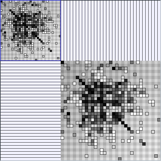
Number of email coded with link width in the nodelink, edge color in the matrix
Email exchange per research group during a week emailGWeek.xml
Number of email coded with link width in the nodelink, edge color in the matrix
Email exchange per research group during a month emailGMonth.xml
Number of email coded with link width in the nodelink, edge color in the matrix
Email exchange per research group during a year emailGYear.xml
Number of email coded with link width in the nodelink, edge color in the matrix
